
Ordination
Mark A. Conaway
Introduction
One of the fundamental tools for visualization in geometric
morphometrics is the Principal Components Analysis (PCA). Users of
geomorph can perform a PCA using the function gm.prcomp. In
addition to a standard PCA, this function can be used to perform a
visualization of phylomorphospace, as well as a phlogenetically-aligned
components analysis (PaCA).
gm.prcomp()
- \(A\): A 3D array (p x k x n) containing Procrustes shape variables for a set of aligned specimens. Alternatively, this can be an n x p matrix of any data, but output will not contain information about shapes.
- \(phy\): An optional phylogenetic tree of class phylo
- \(align.to.phy\): A logical (TRUE or FALSE) argument for whether PaCA (if TRUE) should be performed
- \(GLS\): Whether GLS-centering and covariance estimation should be used (rather than OLS). This argument is FALSE by default.
- \(transform\):
A logical value to indicate if transformed residuals should be projected. This is only applicable if GLS = TRUE. If TRUE, an orthogonal projection of transformed data is made; if FALSE an oblique projection of untransformed data is made.
Principal Components Analysis (PCA)
Running a simple PCA is done similarly to the base R function
prcomp. Summary of the results of this function returns the
eigenvalues, the proportion of variance each eigenvalue accounts for, as
well as the cumulative variance.
PCA <- gm.prcomp(gpa$coords)
summary(PCA)
##
## Ordination type: Principal Component Analysis
## Centering by OLS mean
## Orthogonal projection of OLS residuals
## Number of observations: 9
## Number of vectors 8
##
## Importance of Components:
## Comp1 Comp2 Comp3 Comp4 Comp5 Comp6
## Eigenvalues 0.0002720474 0.0001120524 0.0001084758 0.0000568924 0.0000264508 1.260516e-05
## Proportion of Variance 0.4564029477 0.1879858086 0.1819855633 0.0954461044 0.0443754550 2.114717e-02
## Cumulative Proportion 0.4564029477 0.6443887563 0.8263743196 0.9218204240 0.9661958790 9.873431e-01
## Comp7 Comp8
## Eigenvalues 5.959622e-06 1.584785e-06
## Proportion of Variance 9.998220e-03 2.658730e-03
## Cumulative Proportion 9.973413e-01 1.000000e+00Likewise, one can simply use the base function plot to
generate a bare bones visualization of the results:
plot(PCA, main = "PCA")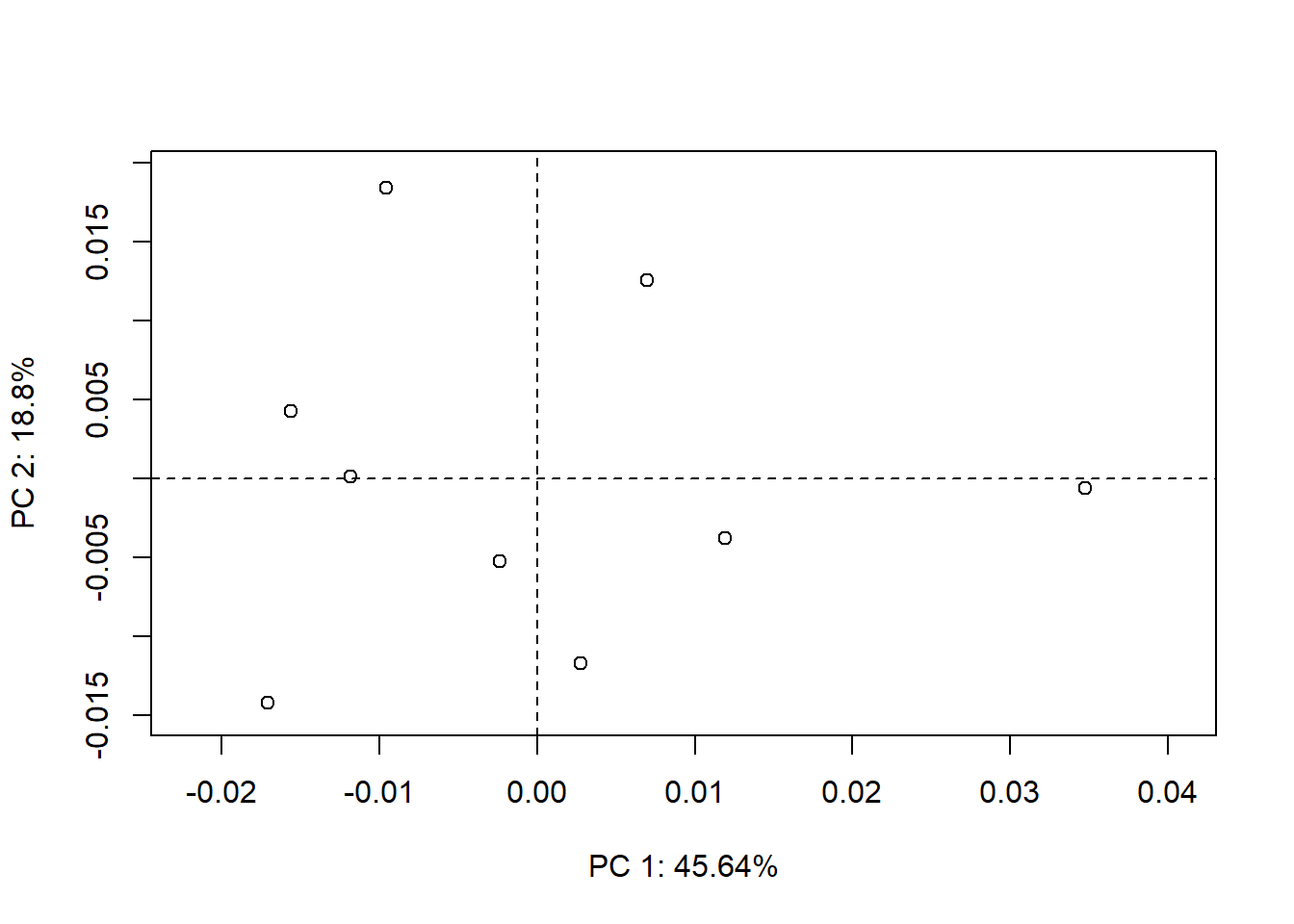
Phylomorphospace
If a PCA is run with an input phylogeny, and the “transform” argument is set to FALSE (as it is by default), the result is the same as a normal PCA, but with estimated ancestral states projected onto the plot.
PCA <- gm.prcomp(gpa$coords, phy = phy, transform = F)
plot(PCA, phylo = T)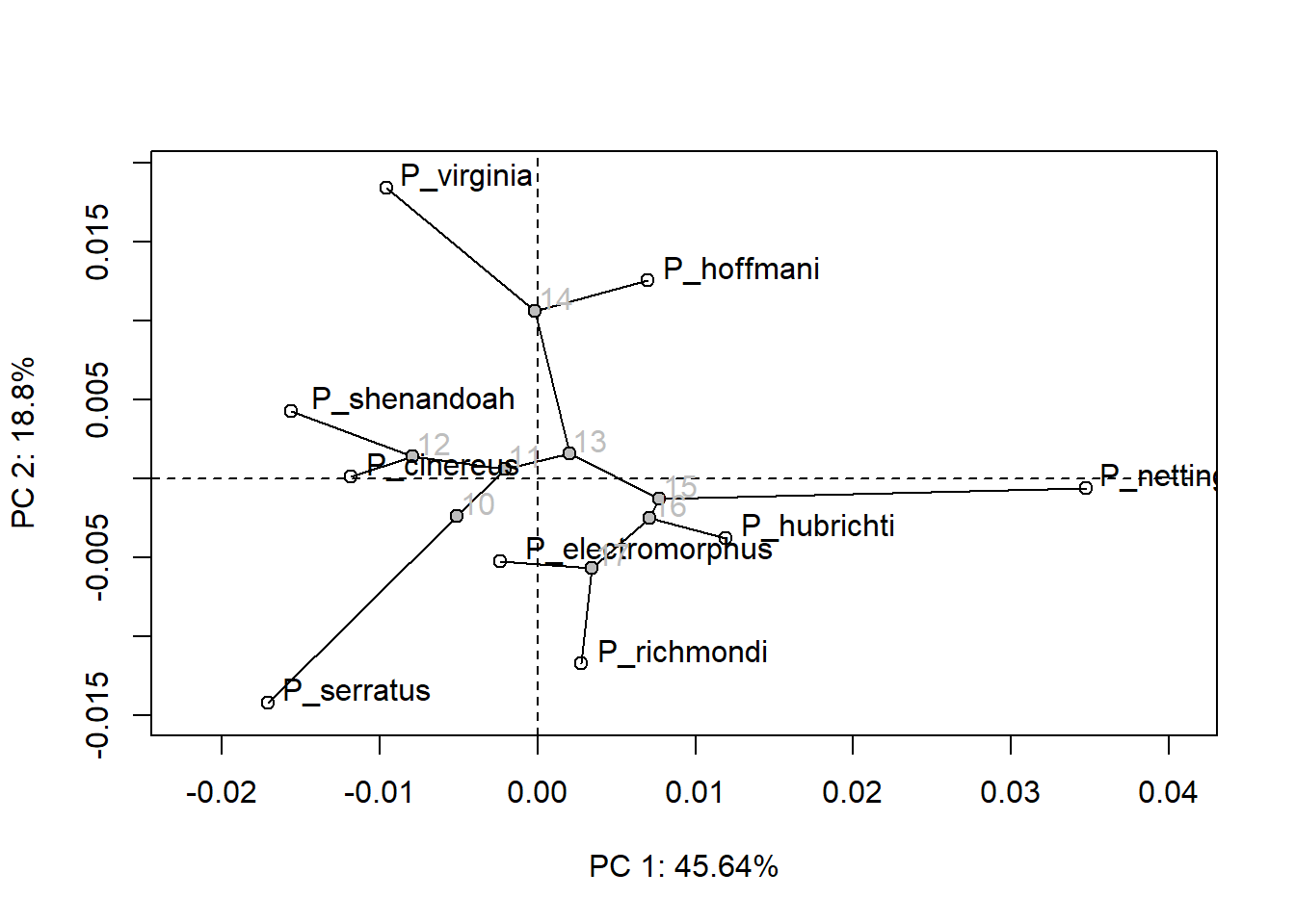
3D phylomorphospace
plot(PCA, time.plot = TRUE, bg = "red",
     phylo.par = list(tip.labels = TRUE,
                      tip.txt.cex = 2, edge.color = "blue", edge.width = 2))
Phylogenetic Principal Components Analysis (phyloPCA)
Following the method of Revell (2009), one can also run a phyloPCA that accounts for non-independence due to phylogeny. This should be run using the GLS method:
PCA <- gm.prcomp(gpa$coords, phy = phy, GLS = T)
plot(PCA, phylo = T)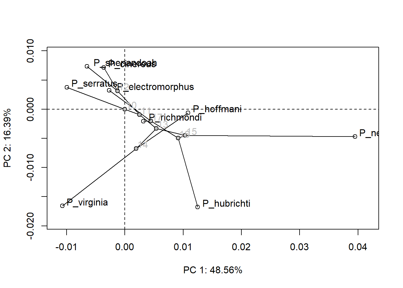
Additionally, the GLS residuals can be transformed, making them independent of the phylogeny:
PCA <- gm.prcomp(gpa$coords, phy = phy, GLS = T, transform = T)
plot(PCA, phylo = T)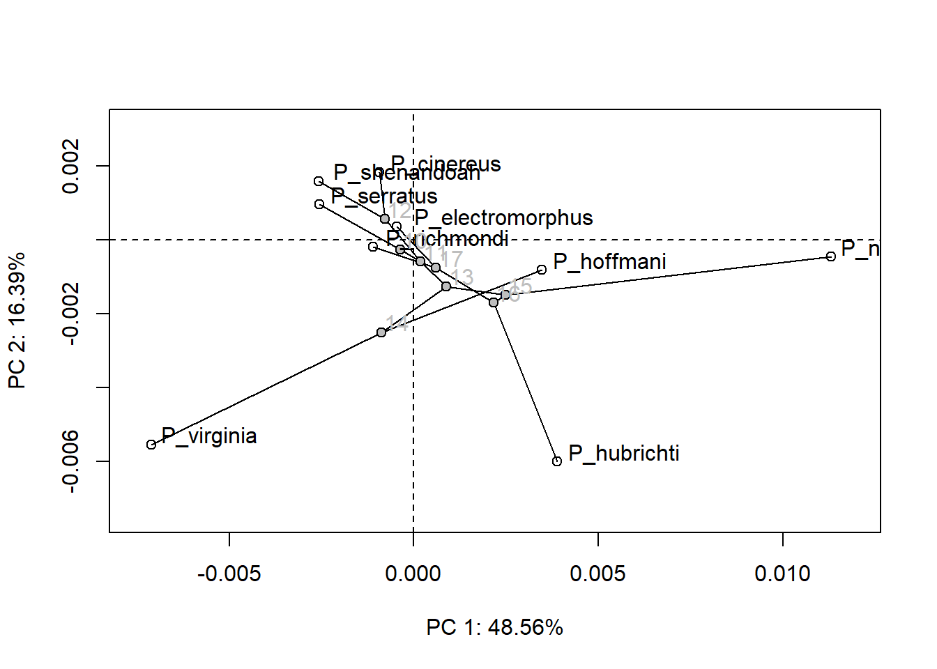
Phylogenetically-aligned Components Analysis (PaCA)
As opposed to a standard PCA, which aligns ones data to an axis of greatest dispersion, the PaCA aligns data to the axis of greatest phylogenetic signal. This can be done with either the GLS or OLS approach. Projection of transformed GLS residuals is possible, but not recommended, since phylogenetic signal is removed from transformed data.
PCA <- gm.prcomp(gpa$coords, phy = phy, align.to.phy = T)
plot(PCA, phylo = T)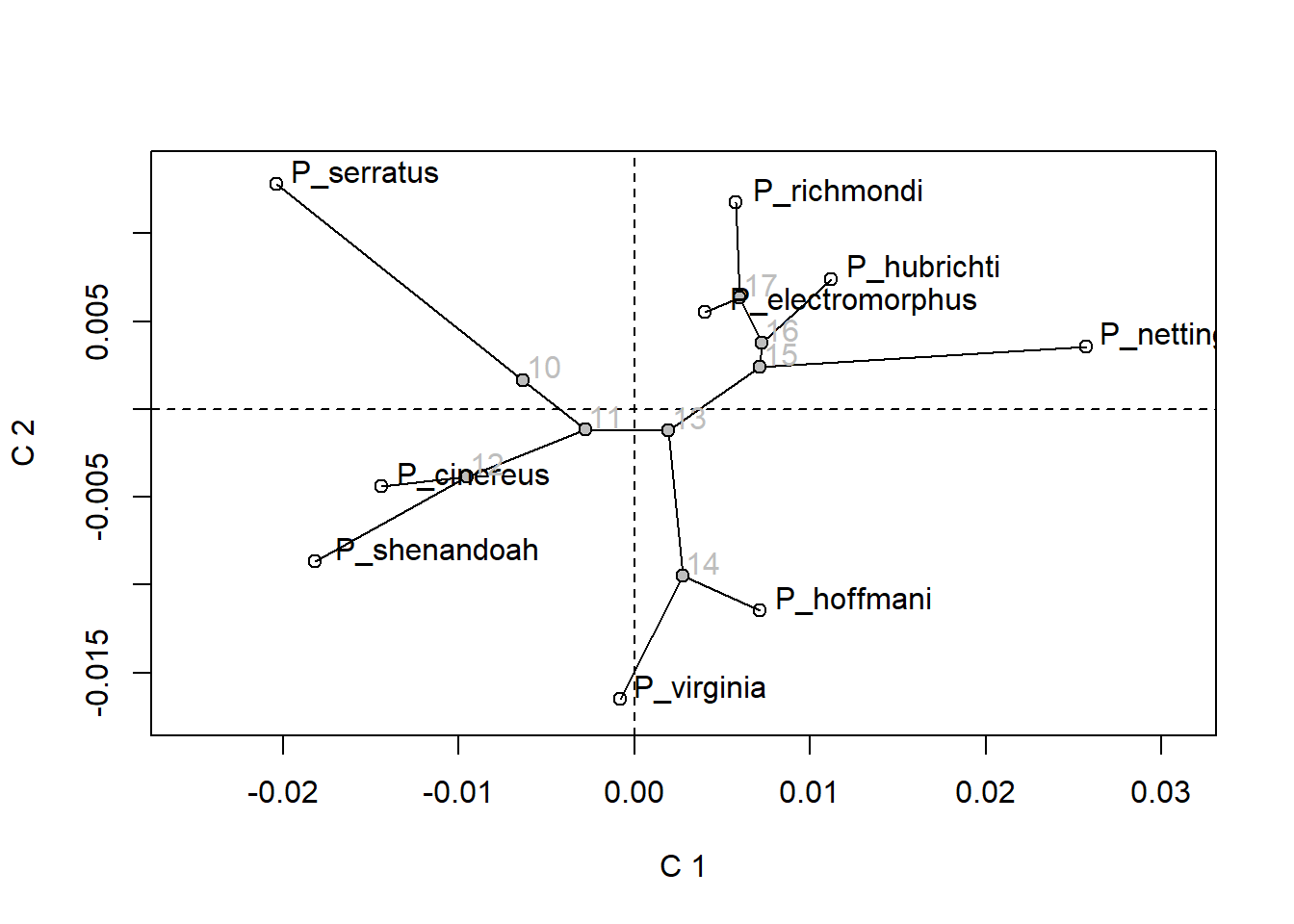
PCA <- gm.prcomp(gpa$coords, phy = phy, align.to.phy = T, GLS = T)
plot(PCA, phylo = T)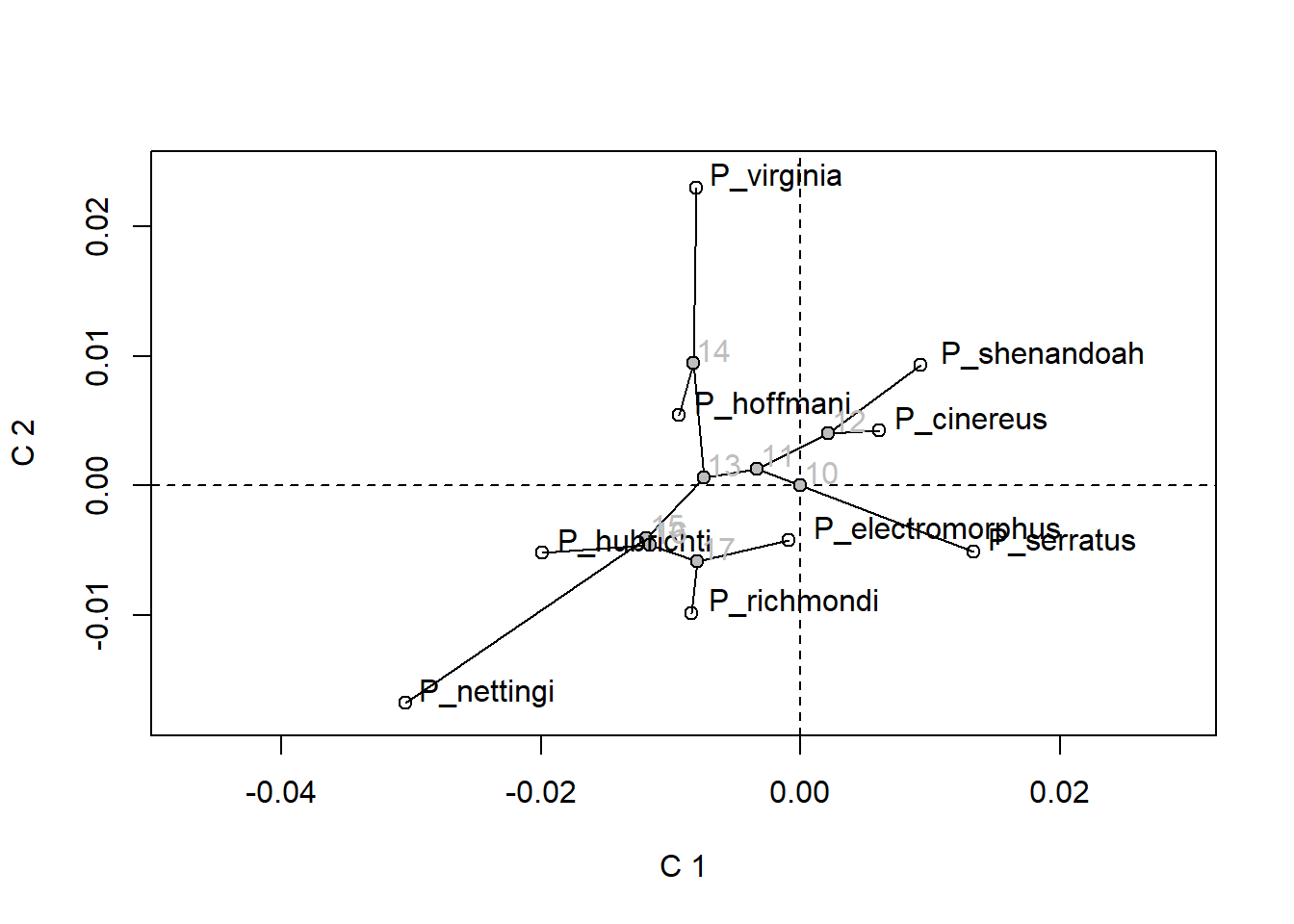
Important Note! For more advanced plotting methods, see the Visualizing Shape Differences workflow tutorial.