Visualizing a Full Landmark Dataset

Introduction

A useful step to visualize patterns of shape variation of a set of specimens (after GPA) is to display all landmark coordinates for all specimens in a single plot. This can be done using the plotAllSpecimens function in geomorph.

plotAllSpecimens()

• \(A\): A 3D array (p x k x n) containing Procrustes shape variables for a set of specimens.
• \(mean\): A logical value (TRUE or FALSE) indicating whether the mean shape should be included in the plot.
• \(links\): An optional matrix defining for links between landmarks (only if mean=TRUE).
• \(label\): A logical value indicating whether landmark numbers will be plotted (only if mean=TRUE).
• \(plot.param\): A list of plot parameters for the points (pt.bg, pt.cex), mean (mean.bg, mean.cex), links (link.col, link.lwd, link.lty) and landmark labels (txt.cex, txt.adj, txt.pos, txt.col).

Plotting two-dimensional landmark data

With two-dimensional data, plotAllSpecimens returns a plot like this:

plotAllSpecimens(gpagen(plethodon$land)$coords)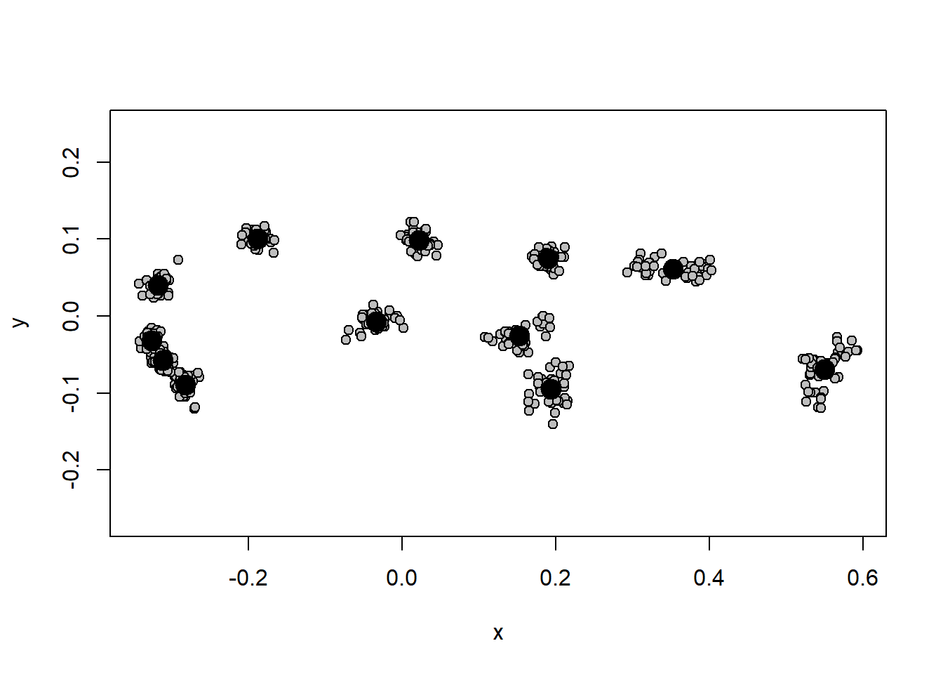

Adding landmark links

Additionally, links between landmarks can be specified in order to generate a wireframe to more easily visualize shape variation. The input for this argument is a matrix of this format:

plethodon$links

##       [,1] [,2]
##  [1,]    4    5
##  [2,]    3    5
##  [3,]    2    4
##  [4,]    1    2
##  [5,]    1    3
##  [6,]    6    7
##  [7,]    7    8
##  [8,]    8    9
##  [9,]    9   10
## [10,]   10   11
## [11,]   11   12
## [12,]   12    1
## [13,]    1    9
## [14,]    1   10

plotAllSpecimens(gpagen(plethodon$land)$coords, links = plethodon$links)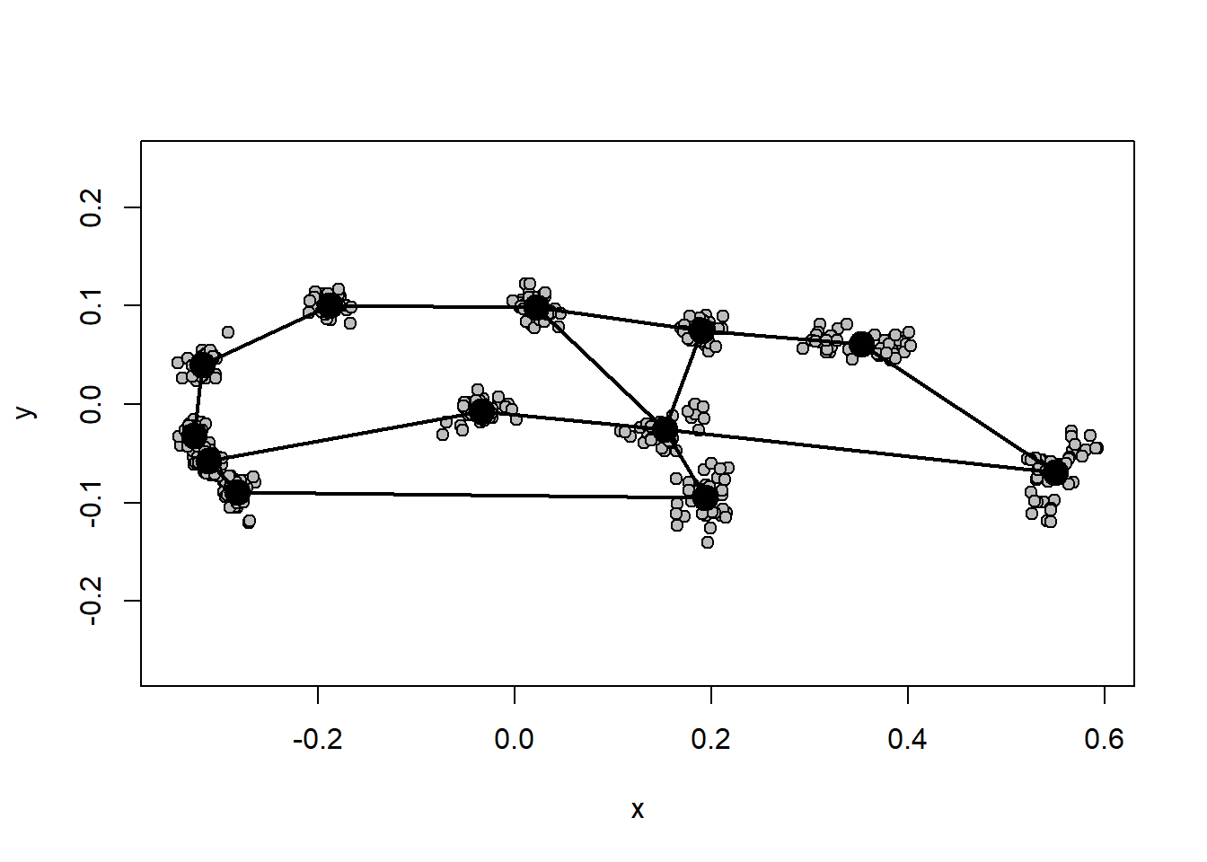

Plotting three-dimensional landmark data

Plotting 3D data is done the same way as with two dimensional data, but the output is an interactive plot that opens automatically in a new window. Links between landmarks can likewise be added to a 3D plot.

plotAllSpecimens(gpagen(scallops$coorddata)$coords)