
Phenotypic Trajectory Analysis
Mark A. Conaway
Introduction
With standard multivariate analyses, such as Procrustes ANOVA, one is able to determine whether shapes differ across one or more variables. However, what this approach lacks is a mechanism whereby one can visualize and understand how shape changes may differ within distinct groups (Collyer & Adams 2013).
Occasionally, when one is working with multiple variables (or factors), levels of one factor (say, sex) may be linked via another factor (population, for example). With multivariate analyses, we can determine whether two variables are related; phenotypic trajectory analysis allows us to determine \(how\) those variables differ. Characteristics of these linkages, representing vectors of change between levels, can be quantified via a phenotypic trajectory analysis. Here, a trajectory refers to a sequence of points within the data space.
To do this, we can use the RRPP function
trajectory.analysis. Note that RRPP is a companion package
which houses the underlying statistical permutational analytics for
geomorph’s statistical procedures. It is installed and loaded
simultaneously with geomorph.
trajectory.analysis()
Allows the user to perform a trajectory analysis on variables of a linear model fit.
- \(fit\): A linear model
fit generated via
procD.lm - \(fit.null\): An alternative linear model fit, if the null model is not desired.
- \(groups\): A factor (or vector that can be changed to a factor) that defines trajectories (see below)
- \(traj.pts\): A single value or factor, to define trajectory points.
- \(pca\): A logical value (TRUE/FALSE) to optionally perform a principal components analysis on a covariance matrix of group:point means. This is only possible when traj.pts is a factor.
- \(print.progress\): Logical value to indicate whether a progress bar should be printed to the screen.
Example Analysis
For the purposes of this example, generating a model fit using the
procD.lm function will be taken as-read. If you are not
familiar with the procD.lm function please see the ANOVA/Regression tutorial before proceeding here. Below is
an example analysis of sexual dimorphism vectors of pupfish, the dataset
for which is included by default with geomorph.
data(Pupfish)
fit <- procD.lm(coords ~ Pop * Sex, data = Pupfish, iter = 999, print.progress = FALSE)
TA <- trajectory.analysis(fit, groups = Pupfish$Pop, traj.pts = Pupfish$Sex)Results of this analysis can be summarized in different ways:
The magnitude difference between path distancessummary(TA, attribute = "MD")##
## Trajectory analysis
##
## 1000 permutations.
##
## Points projected onto trajectory PCs
##
## Trajectories:
## Trajectories hidden (use show.trajectories = TRUE to view)
##
## Observed path distances by group
##
## Marsh Sinkhole
## 0.04611590 0.02568508
##
## Pairwise absolute differences in path distances, plus statistics
## d UCL (95%) Z Pr > d
## Marsh:Sinkhole 0.02043082 0.01279423 2.660878 0.001summary(TA, attribute = "TC", angle.type = "deg")##
## Trajectory analysis
##
## 1000 permutations.
##
## Points projected onto trajectory PCs
##
## Trajectories:
## Trajectories hidden (use show.trajectories = TRUE to view)
##
## Pairwise correlations between trajectories, plus statistics
## r angle UCL (95%) Z Pr > angle
## Marsh:Sinkhole 0.7393716 42.32209 22.06859 3.766063 0.001Finally, results can be plotted to aid visualization. Vector length describes how much shape change occurs per unit change of size, and the vector directions describe the relative covariation of shape variables per unit change of size.
TP <- plot(TA, pch = as.numeric(Pupfish$Pop) + 20, bg = as.numeric(Pupfish$Sex),
           cex = 0.7, col = "gray")
add.trajectories(TP, traj.pch = c(21, 22), start.bg = 1, end.bg = 2)
legend("topright", levels(Pupfish$Pop), pch =  c(21, 22), pt.bg = 1)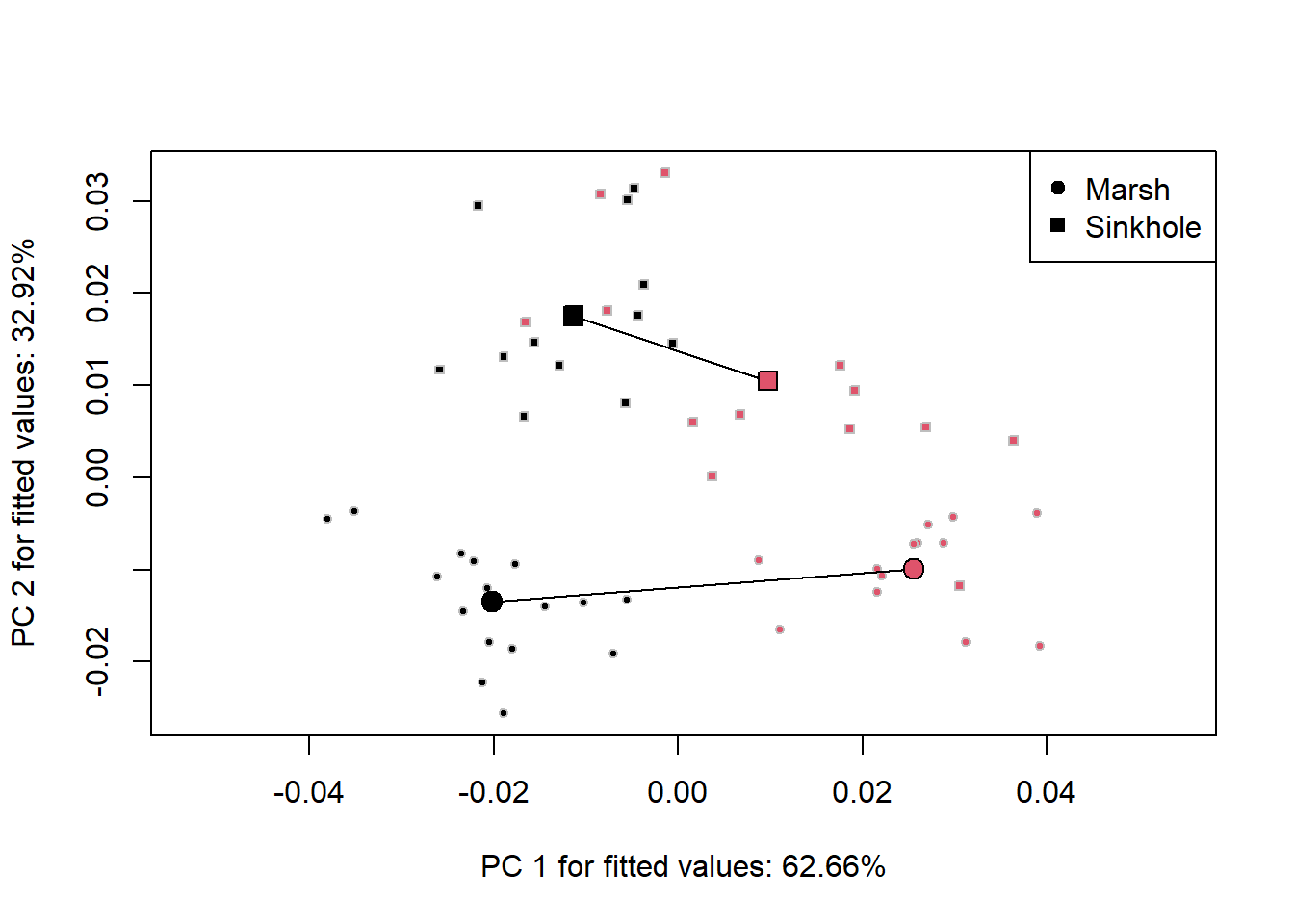
The values for each permutation of the above measures, along with other information, can be accessed in the object of class “trajectory.analysis” that is created from this function:
trajectory.analysis Output
- \(LS.means\): Least-squares means
from the
pairwisefunction - \(trajectories\): Trajectories from every permutation.
- \(PD\): Permutation values of path distances of trajectories
- \(MD\): Permutation values of magnitude differences between trajectories.
- \(TC\): Permutation values of trajectory correlations
- \(SD\): Permutation values of shape difference between trajectories