
Comparing Rates of Shape Evolution on Phylogenies (Single Trait)
Mark A. Conaway
Introduction: Phylogenetic Comparative Methods
Fitting linear models, and performing statistical analyses in
general, to assess biological hypotheses regarding closely-related
species presents a problem to the researcher. Standard statistical
models rely on the assumption that observations are independent and
identically distributed (iid). Mathematically, this means that the
Gaussian error of an iid dataset can be expressed as an identity matrix.
However, when species are closely related (for example within the same
genus) by phylogeny, we expect observations taken on them to be more
similar than those taken from more distantly-related species. This means
that error in this case cannot be expressed as an identity matrix. In
other words, observations taken from closely related species cannot be
considered independent, or identically distributed. Phylogenetic
Comparative Methods (PCM) is an analytical toolkit consisting of
methodologies designed to account for this issue of non-independence of
observations. With this toolkit, researchers can construct models and
perform other related analyses with non independent observations by
subsequently \(conditioning\) those
observations on a phylogeny. Under this PCM analytical umbrella are Phylogenetic ANOVA, Phylomorphospace, Phylogenetic Signal, and Evolutionary Rates,
all of which can be performed using functions in
geomorph.
Comparing Evolutionary Rate Among Traits
The compare.multi.evol.rates function, allows the user
to calculate and compare rates of evolution on a phylogeny among sets of
variables for the same set of species. This function follows the
protocol of Denton & Adams (2015) whereby, after the data (a 3D array of Procrustes coordinates) are conditioned on the
phylogeny, the net rate of shape evolution for each provided trait is
calculated, and a ratio obtained. Finally evolutionary rates are
compared based on the outer-product matrix of between-species
differences after phylogenetic transformation. This ratio, if three or
more traits are input, is defined as the ratio of the maximum to minimum
rate.
compare.multi.evol.rates()
- \(A\): A 3D array (p x k x n) containing GPA-aligned coordinates for all specimens, or a matrix (n x variables)
- \(gp\): A factor array designating group membership for individuals
- \(phy\): A phylogenetic tree of class phylo - see read.tree in library ape
- \(subset\): A logical value indicating whether or not the traits are subsets from a single landmark configuration (default is TRUE)
- \(iter\): Number of iterations for significance testing
- \(seed\): An optional argument for setting the seed for random permutations of the resampling procedure. If left NULL (the default), the exact same P-values will be found for repeated runs of the analysis (with the same number of iterations). If seed = “random”, a random seed will be used, and P-values will vary. One can also specify an integer for specific seed values, which might be of interest for advanced users.
- \(print.progress\): A logical value to indicate whether a progress bar should be printed to the screen. This is helpful for long-running analyses.
Example Analysis
To illustrate the use of this function, we will compare evolutionary rates between two sets of traits of plethodon salamanders crania. The data used here are available with geomorph as part of the ‘plethspecies’ dataset.
First, we must create a vector that will be used to identify which landmarks belong to which group:land.gp<-c("A","A","A","A","A","B","B","B","B","B","B") EMR<-compare.multi.evol.rates(A = lmks$coords,gp = land.gp,
Subset = TRUE, phy = plethspecies$phy,iter=999, print.progress = F)summary:
summary(EMR)##
## Call:
##
##
## Observed Rate Ratio: 1.2997
##
## P-value: 0.468
##
## Effect Size: 0.11
##
## Based on 1000 random permutations
##
## The rate for group A is 1.97486252507008e-06
##
## The rate for group B is 2.56682040817109e-06plot:
plot(EMR)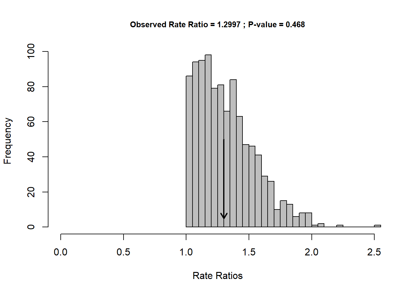
This function generates an object of class “evolrate” which is a list, whose objects can be accessed using the $ operator.
compare.evol.rates() Output
- \(rates.all\): The phylogenetic evolutionary rates for each trait.
- \(rate.ratio\): The ratio of maximum to minimum evolutionary rates.
- \(pvalue\): The significance level of the observed rate ratio.
- \(Effect.Size\): The multivariate effect size associated with sigma.d.ratio.
- \(pvalue.gps\): Matrix of pairwise significance levels comparing each pair of rates.
- \(call\): The matched call.
Important Note! To compare evolutionary rates among
different \(groups\) (as opposed to
traits), see the tutorial for compare.evol.rates