
Phylogenetic Modularity
Mark A. Conaway & Dean C. Adams
Introduction
As with other analytical methods covered in these
tutorials, similarity due to phylogeny will often need to be accounted
for in analyses of modularity. The function
phylo.modularity quantifies the degree of phylogenetic
modularity in two or more hypothesized modules of Procrustes shape
variables as defined by landmark coordinates, under a Brownian motion
model of evolution. The degree of modularity is characterized by the
covariance ratio covariance ratio (CR: see Adams 2016). This function is
an extension of the modularity.test function in the same
way that phylo.integration is an extension of integration.test. As with these other functions, input for
this function can be either multiple objects containing Procrustes
coordinates, or a single object along with a vector used to define
partitions.
For this analysis, the phylogenetic relationships among taxa are
described by the phylogeny, which in R is an object of class “phylo”.
Note that there is a slight difference between geomorph and
RRPP in how phylogenetic information is provided by the
user. In geomorph, phylogenetic information is generally provided as a
phylogeny of class “phylo”. This object is then converted to a
phylogenetic covariance matrix by the internal analytics of the
function. By contrast, in RRPP the user must first calculate the
phylogenetic covariance matrix, and then provide this to the analytical
functions to incorporate phylogenetic information. Users should be aware
of this slight difference, as several geomorph functions
call underlying RRPP functions (e.g.,
procD.pgls in geomorph calls lm.rrpp in
RRPP).
phylo.modularity()
- \(A\): A 2D array (n x [p1 x k1]) or 3D array (p1 x k1 x n) containing Procrustes shape variables for the first block
- \(phy\): A phylogenetic tree of class phylo
- \(CI\): A logical argument indicating whether bootstrapping should be used for estimating confidence intervals
- \(partition.gp\): A list of which landmarks (or variables) belong in which partition: (e.g. A, A, A, B, B, B, C, C, C). Required when only one dataset is provided.
- \(iter\): Number of iterations for significance testing
- \(seed\): An optional argument for setting the seed for random permutations of the resampling procedure. If left NULL (the default), the exact same P-values will be found for repeated runs of the analysis (with the same number of iterations). If seed = “random”, a random seed will be used, and P-values will vary. One can also specify an integer for specific seed values, which might be of interest for advanced users.
- \(print.progress\): A logical (TRUE/FALSE) value to indicate whether a progress bar should be printed to the screen. This is helpful for long-running analyses.
Example of Analysis of Phylogenetic Modularity
For this example, we first create a vector (lmkpart) that defines the
partitions of our data. Then we run the analyses, including our
phylogeny as an argument of the function. The phylogenetic tree and
landmarks included in this example are from the “plethspecies” dataset,
available by default with geomorph.
lmkpart <- c("A","A","A","A","A","B","B","B","B","B","B")
MT <- phylo.modularity(lmks$coords, phy = phylo, partition.gp=lmkpart, CI = F, iter=999, print.progress = F)
Just like with the function modularity.test, results can
be summarized using the base R function summary. Likewise,
the base R function plot can be used to generate a
histogram of coefficients obtained via resampling is presented, with the
observed value designated by an arrow in the plot.
summary(MT) ##
## Call:
## phylo.modularity(A = lmks$coords, partition.gp = lmkpart, phy = phylo,
## CI = F, iter = 999, print.progress = F)
##
##
##
## CR: 1.1625
##
## P-value: 0.683
##
## Effect Size: 0.3738
##
## Based on 1000 random permutationsplot(MT)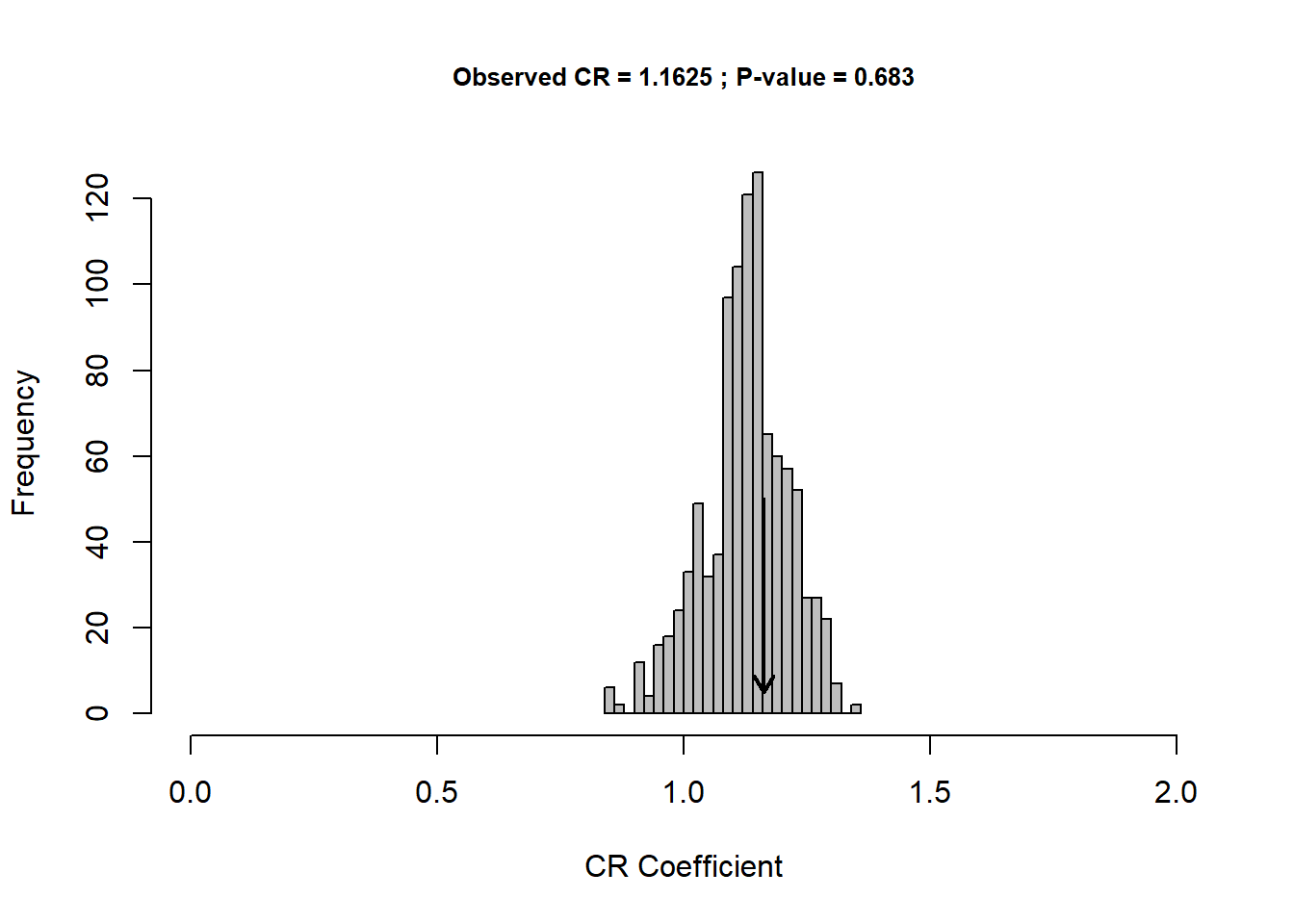
This function returns an object of class “CR”, which is a list containing the following:
phylo.modularity output
- \(CR\): Covariance ratio: The estimate of the observed modular signal.
- \(CInterval\): The bootstrapped 95 percent confidence intervals of the CR, if CI = TRUE.
- \(CR.boot\): The bootstrapped CR values, if CI = TRUE
- \(P.value\): The empirically calculated P-value from the resampling procedure.
- \(Effect.Size\): The multivariate effect size associated with sigma.d.ratio.
- \(CR.mat\): For more than two partitions, the pairwise CRs among partitions.
- \(random.CR\): The CR calculated in each of the random permutations of the resampling procedure.
- \(Pcov\): The phylogenetic transformation matrix, needed for certain other analyses.
- \(permutations\): The number of random permutations used in the resampling procedure.
- \(call\): The match call (input code).