
Obtaining Symmetric Shapes
Mark A. Conaway
Introduction
Many biological objects display some sort of symmetry. Morphometric analyses often investigate symmetry in some manner: either by evaluating components of variation attributed to different symmetry effects (e.g., directional, fluctuating, etc.), or by accounting for symmetry prior to the analysis (e.g., obtain ‘symmetrized’ shapes for subsequent investigation). This tutorial will focus on the latter, and give an overview of the preliminary steps necessary for generation of symmetric shapes. Analyses of asymmetry are covered in a separate tutorial.
This tutorial will utilize the function bilat.symmetry.
The function will be described in much greater detail in the [asymmetry
tutorial], as well as the advanced options page, but all
relevant arguments and outputs for the removal of asymmetric shape
components will be described here.
bilat.symmetry() (Expand for more details)
\(A\): A 3D array of either raw, or Procrustes-aligned landmark coordinates OR a
gpagenobject, that is, the output from thegpagenfunction.\(ind\): A vector containing labels for each individual:
lizards$ind## [1] 29 29 30 30 31 31 32 32 33 33 34 34 35 35 36 36 37 37 38 38 39 39 40 40 41 41 42 42 43 43 44 44 45 45 46
## [36] 46 47 47 48 48 49 49 50 50 51 51 52 52 53 53 54 54 55 55 56 56 57 57 58 58 59 59 60 60 61 61 62 62 63 63
## [71] 64 64 65 65 66 66 67 67 68 68 69 69 70 70 71 71 72 72 73 73 74 74 75 75 76 76 77 77Here, the levels indicate different individuals, whose landmarks on
sided elements have been repeated.
- \(replicate\): A vector that identifies which objects belong to which group of replicates:
lizards$rep## [1] 1 2 1 2 1 2 1 2 1 2 1 2 1 2 1 2 1 2 1 2 1 2 1 2 1 2 1 2 1 2 1 2 1 2 1 2 1 2 1 2 1 2 1 2 1 2 1 2 1 2 1 2 1
## [54] 2 1 2 1 2 1 2 1 2 1 2 1 2 1 2 1 2 1 2 1 2 1 2 1 2 1 2 1 2 1 2 1 2 1 2 1 2 1 2 1 2 1 2 1 2\(object.sym\): Since these data are an example of object symmetry, this argument is set to TRUE.
\(land.pairs\): In the case of object symmetry, this argument contains a matrix indicating numbers for matched pairs of landmarks across the line of symmetry:
lizards$lm.pairs## [,1] [,2]
## [1,] 13 14
## [2,] 2 11
## [3,] 15 16
## [4,] 27 28
## [5,] 3 10
## [6,] 17 19
## [7,] 4 9
## [8,] 20 21
## [9,] 22 24
## [10,] 5 8
## [11,] 6 7
## [12,] 25 26Input
Let’s start with the lizards dataset embedded in
geomorph; data that are an example of object symmetry:
lizard.sym <- bilat.symmetry(lizards$coords, ind = lizards$ind,
                             replicate = lizards$rep, object.sym = TRUE,
                             land.pairs = lizards$lm.pairs, print.progress = FALSE)
Output
The output of bilat.symmetry is a large list, most of
the components of which are discussed [elsewhere]. For the moment we are
interested in extracting the symmetric shape components from our data.
In the first place, these components can be illustrated simply by
plotting our bilat.symmetry object:
plot(lizard.sym)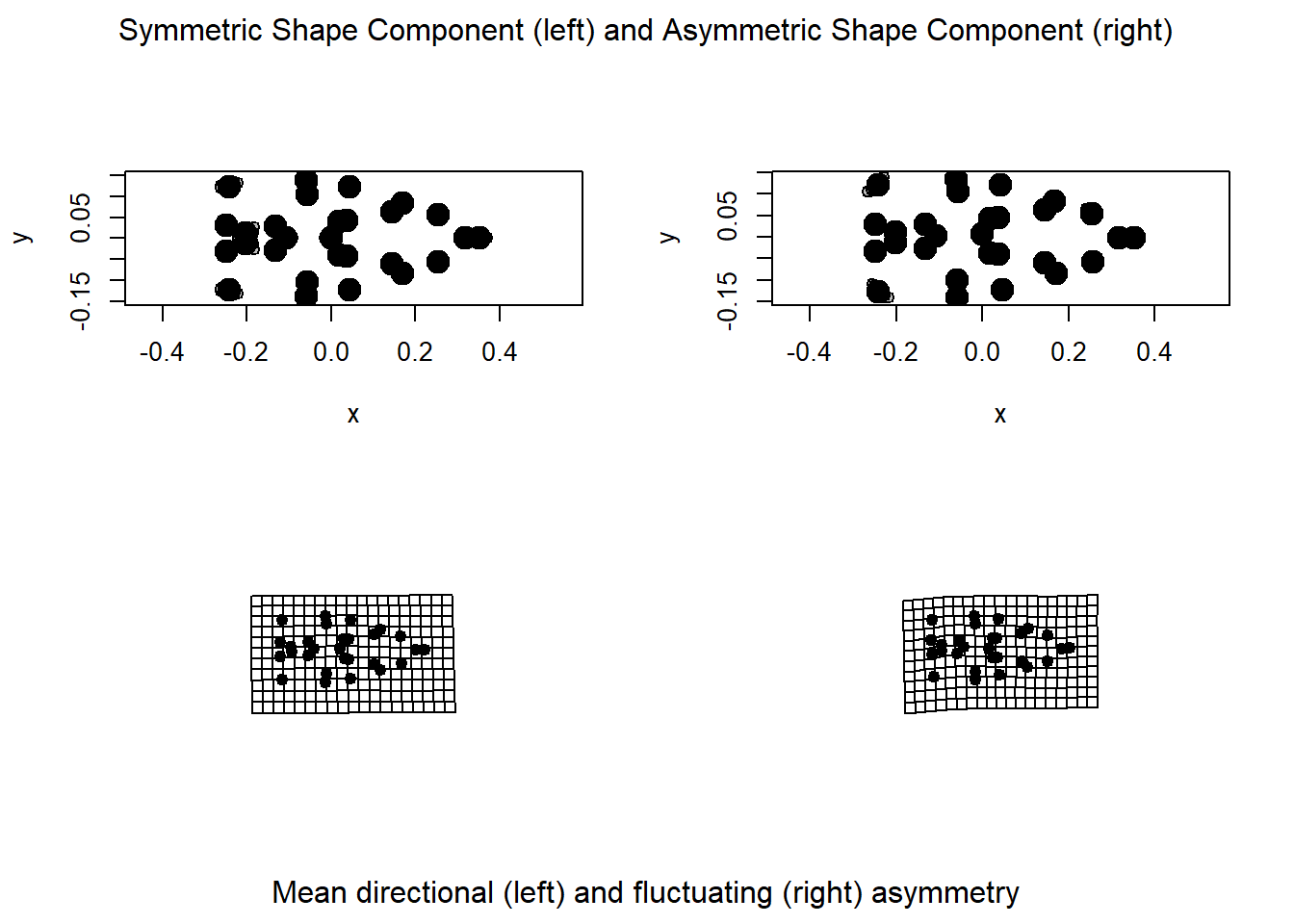
The symmetric shape component of our data can be accessed with the following code:
lizard.sym$symm.shapeThe symm.shape subset of our results is a 3D array of coordinates
representing the symmetric component of shape variation that can then be
used for further analyses.