
Global Integration
Mark A. Conaway
Introduction
An alternative method for quantifying morphological integration is
the “Global integration” as put forth by Bookstein (2015). This method
estimates the set of bending energies of a set of aligned specimens at
various spatial scales, and plots the log of the variance of the partial
warps versus the log of their corresponding bending energies. This can
be accomplished using the geomorph function
globalIntegration
A slope of negative one corresponds to self-similarity, implying that patterns of shape variation are similar across spatial scales. Steeper slopes (i.e., those more extreme than -1.0) correspond to data that are globally integrated, while shallower slopes (between -1 and 0) correspond to data that are ’disintegrated (see Bookstein 2015). Isotropic data will have an expected slope of zero.
globalIntegration()
- \(A\): 3D array (p1 x k x n) containing Procrustes shape variables
- \(ShowPlot\): A logical (TRUE/FALSE) value indicating whether or not the plot should be returned
Example of Analysis of Global Integration
Below is example code using the “plethodon” dataset, included by
default with the geomorph package.
int <- globalIntegration(lmks$coords)

int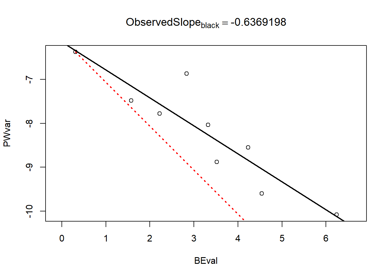
##      BEval
## -0.6369198