
Two-block Partial Least Squares Analysis
Mark A. Conaway
Introduction
A two-block partial least squares (PLS) analysis is useful when one
wishes to quantify the degree of association (covariance) between two
sets of variables. A PLS analysis has characteristics similar to that of
linear regression in that the result of an analysis is linear
combinations of variables. Likewise, however, PLS maintains some
characteristics similar to ordination methods such as PCA, in that the
result is mutually orthogonal axes derived from a covariance matrix. The
difference is that, the axes generated from a PLS analysis describe
covariance between the two input data sets, rather than variance, and
are derived from an inter-block covariance matrix. In
geomorph, can perform a PLS analysis between sets of
Procrustes variables (or other variables) using the
two.b.pls function.
two.b.pls()
- \(A1\): A 3D array (p x k x n) containing Procrustes shape variables for the first block, or a matrix (n x variables)
- \(A2\): A 3D array (p x k x n) containing Procrustes shape variables for the second block, or a matrix (n x variables)
- \(iter\): Number of iterations for significance testing
- \(seed\): An optional argument for setting the seed for random permutations of the resampling procedure. If left NULL (the default), the exact same P-values will be found for repeated runs of the analysis (with the same number of iterations). If seed = “random”, a random seed will be used, and P-values will vary. One can also specify an integer for specific seed values, which might be of interest for advanced users.
- \(print.progress\): A logical (TRUE/FALSE) value to indicate whether a progress bar should be printed to the screen. This is helpful for long-running analyses.
Example of Analysis
Below is example code using the “plethShapeFood” dataset, included by
default with geomorph.
PLS <- two.b.pls(gpa$coords, food, iter = 999, print.progress = F)
summary(PLS)
##
## Call:
## two.b.pls(A1 = gpa$coords, A2 = food, iter = 999, print.progress = F)
##
##
##
## r-PLS: 0.759
##
## Effect Size (Z): 3.8842
##
## P-value: 0.001
##
## Based on 1000 random permutationsplot(PLS)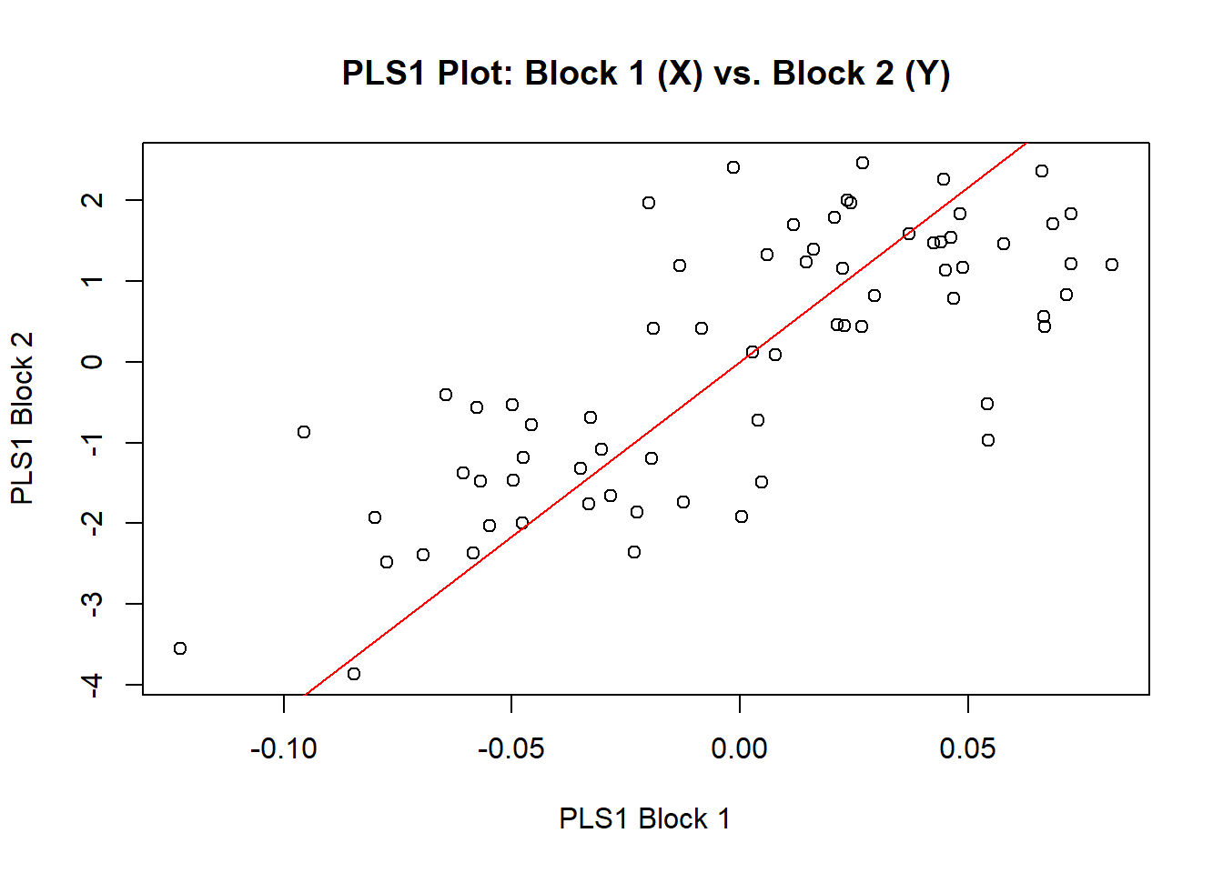
Results of multiple two-block comparisons made with
two.b.pls can be compared using the compare.pls function in geomorph. Note that
this function is also used to compare results of the
integration.test and phylo.integration
functions which are addressed in other tutorials.
PLS1 <- two.b.pls(gpa$coords[,,1:30], food[1:30,], iter = 999, print.progress = F)
PLS2 <- two.b.pls(gpa$coords[,,31:69], food[31:69,], iter = 999, print.progress = F)
compare <- compare.pls(PLS1,PLS2)
summary(compare)##
## Effect sizes
##
## PLS1 PLS2
## -0.6627612 1.9864493
##
## Effect sizes for pairwise differences in PLS effect size
##
## PLS1 PLS2
## PLS1 0.000000 2.037695
## PLS2 2.037695 0.000000
##
## P-values
##
## PLS1 PLS2
## PLS1 1.00000000 0.04158041
## PLS2 0.04158041 1.00000000To perform a similar analysis with a single function, see the tutorial for integration.test.
two.b.pls Output
This function returns an object of class “pls” that contains the following values, each of which can be accessed with the $ operator.
- \(r.pls\): The correlation coefficient between scores of projected values on the first singular vectors of left (x) and right (y) blocks of landmarks (or other variables). This value can only be negative if single variables are input, as it reduces to the Pearson correlation coefficient.
- \(P.value\): The empirically calculated P-value from the resampling procedure.
- \(Effect.Size\): The multivariate effect size associated with sigma.d.ratio.
- \(left.pls.vectors\): The singular vectors of the left (x) block
- \(right.pls.vectors\): The singular vectors of the right (y) block
- \(random.r\): The correlation coefficients found in each random permutation of the resampling procedure.
- \(XScores\): Values of left (x) block projected onto singular vectors.
- \(YScores\): Values of right (y) block projected onto singular vectors.
- \(svd\): The singular value decomposition of the cross-covariances.
- \(A1\): Input values for the left block.
- \(A2\): Input values for the right block.
- \(A1.matrix\): Left block (matrix) found from A1.
- \(A2.matrix\):Right block (matrix) found from A2.
- \(permutations\): The number of random permutations used in the resampling procedure.
- \(call\): The match call.
Important Note! If one wishes to incorporate a phylogeny in a PLS analysis, please see the tutorial for the phylo.integration function.