
Phylogenetic Signal in Shape Variables
Mark A. Conaway
Introduction: Phylogenetic Comparative Methods
Fitting linear models, and performing statistical analyses in
general, to assess biological hypotheses regarding closely-related
species presents a problem to the researcher. Standard statistical
models rely on the assumption that observations are independent and
identically distributed (iid). Mathematically, this means that the
Gaussian error of an iid dataset can be expressed as an identity matrix.
However, when species are closely related (for example within the same
genus) by phylogeny, we expect observations taken on them to be more
similar than those taken from more distantly-related species. This means
that error in this case cannot be expressed as an identity matrix. In
other words, observations taken from closely related species cannot be
considered independent, or identically distributed. Phylogenetic
Comparative Methods (PCM) is an analytical toolkit consisting of
methodologies designed to account for this issue of non-independence of
observations. With this toolkit, researchers can construct models and
perform other related analyses with non independent observations by
subsequently \(conditioning\) those
observations on a phylogeny. Under this PCM analytical umbrella are Phylogenetic ANOVA, Phylomorphospace, Phylogenetic Signal, and Evolutionary Rates,
all of which can be performed using functions in
geomorph.
Phylogenetic Signal
Phylogenetic signal refers to the extent to which phenotypic similarity in a dataset is associated with phylogenetic relatedness. This signal is expected to be higher among the most closely-related species but, in cases where relationships among species are not as close, but still potentially significant, phylogenetic signal can be used to determine whether one’s subsequent analyses should take phylogeny into account (Adams, 2014). Perhaps more importantly, quantifying phylogenetic signal across several traits can help to show which aspects of the phenotype are more evolutionarily labile.
The physignal function in geomorph utilizes a
multivariate version of the K-statistic (Blomberg etal., 2003; Adams,
2014). This is achieved via a distance-based formulation rather than a
covariance-based one. In other words, this function calculates
phylogenetic signal as the ratio of the Euclidean distance between each
species (the observed variation) and the distance between each species
and the origin of the phylogeny (variation accounting for phylogeny),
divided by the ratio of the variation expected under Brownian motion,
relative to the number of taxa in the phylogeny (Adams, 2014).
Significance of this statistic is computed by permuting the shape data
among the tips of the phylogeny.
While physignal is designed for multivariate data,
univariate data can be input as well if imported as a matrix with row
names giving the taxa names. For univariate data, the standard
K-statistic is calculated.
physignal()
- \(A\): A 3D array (p x k x n) containing GPA-aligned coordinates for all specimens, or a matrix (n x variables)
- \(phy\): A phylogenetic tree of class phylo - see read.tree in library ape
- \(iter\): Number of iterations for significance testing
- \(seed\): An optional argument for setting the seed for random permutations of the resampling procedure. If left NULL (the default), the exact same P-values will be found for repeated runs of the analysis (with the same number of iterations). If seed = “random”, a random seed will be used, and P-values will vary. One can also specify an integer for specific seed values, which might be of interest for advanced users.
- \(print.progress\): A logical value to indicate whether a progress bar should be printed to the screen. This is helpful for long-running analyses.
Example Analysis: Phylogenetic Signal in Shape
To illustrate the use of this function, we test for phylogenetic signal in the head shape of plethodon salamanders. The data used here are available with geomorph as part of the ‘plethspecies’ dataset.
PS.shape <- physignal(A = lmks$coords, phy = plethspecies$phy, iter=999)summary:
summary(PS.shape)##
## Call:
## physignal(A = lmks$coords, phy = plethspecies$phy, iter = 999)
##
##
##
## Observed Phylogenetic Signal (K): 0.9573
##
## P-value: 0.008
##
## Based on 1000 random permutations
##
## Use physignal.z to estimate effect size.plot:
plot(PS.shape)
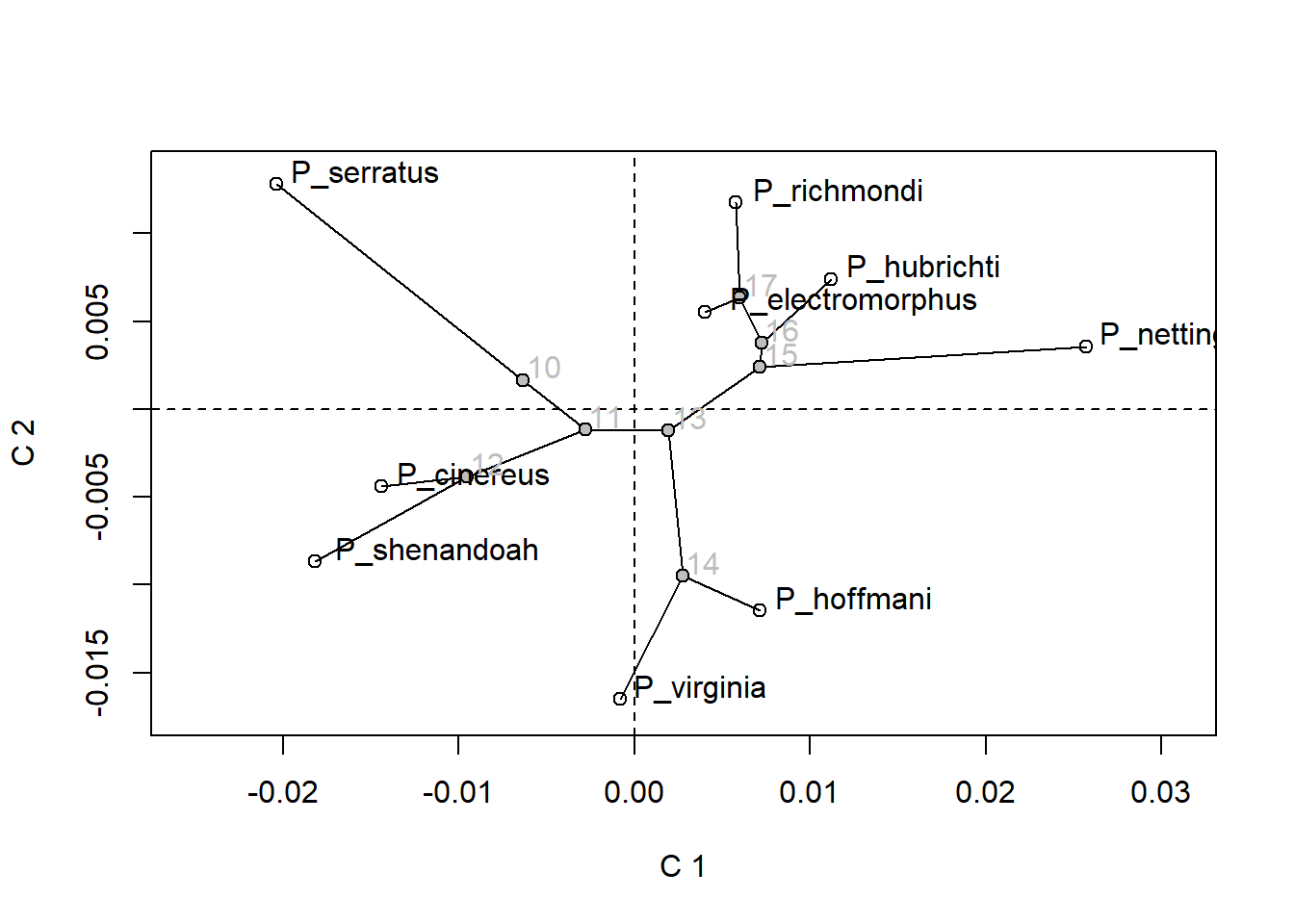
plot(PS.shape$PACA, phylo = TRUE)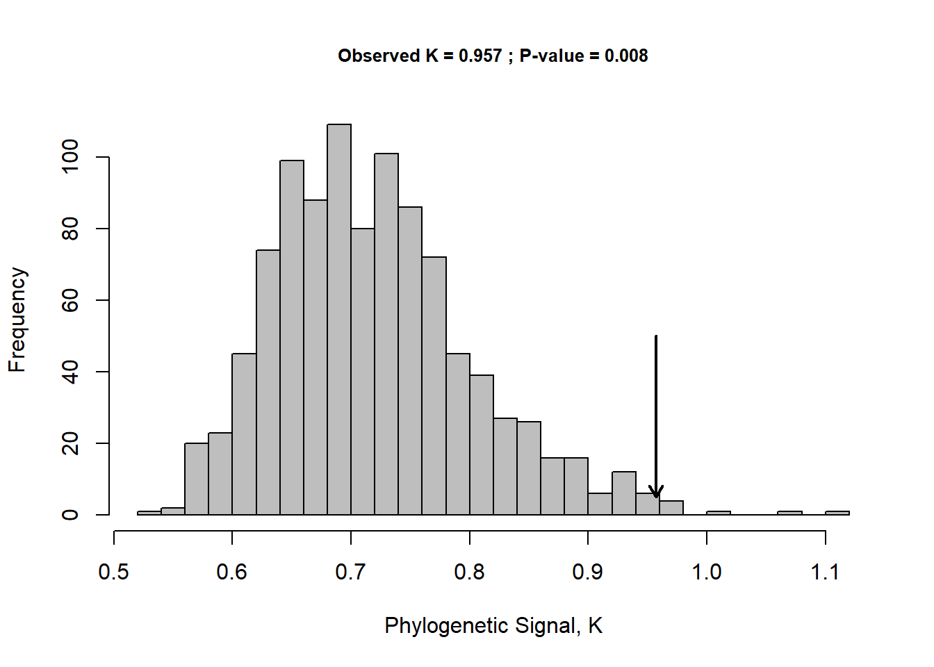
PS.shape$K.by.p## [1] 1.5034858 1.4253457 1.1610972 1.0762048 1.0010464 0.9746155 0.9623519 0.9572991 0.9572991Example Analysis: Phylogenetic Signal in Size
To quantify the phylogenetic signal of size, simple replace the Procrustes coordinates in the ‘A’ argument with the centroid size of one’s data ($Csize):
PS.size <- physignal(A = lmks$Csize, phy = plethspecies$phy, iter=999)summary(PS.size)##
## Call:
## physignal(A = lmks$Csize, phy = plethspecies$phy, iter = 999)
##
##
##
## Observed Phylogenetic Signal (K): 0.7098
##
## P-value: 0.477
##
## Based on 1000 random permutations
##
## Use physignal.z to estimate effect size.plot(PS.size)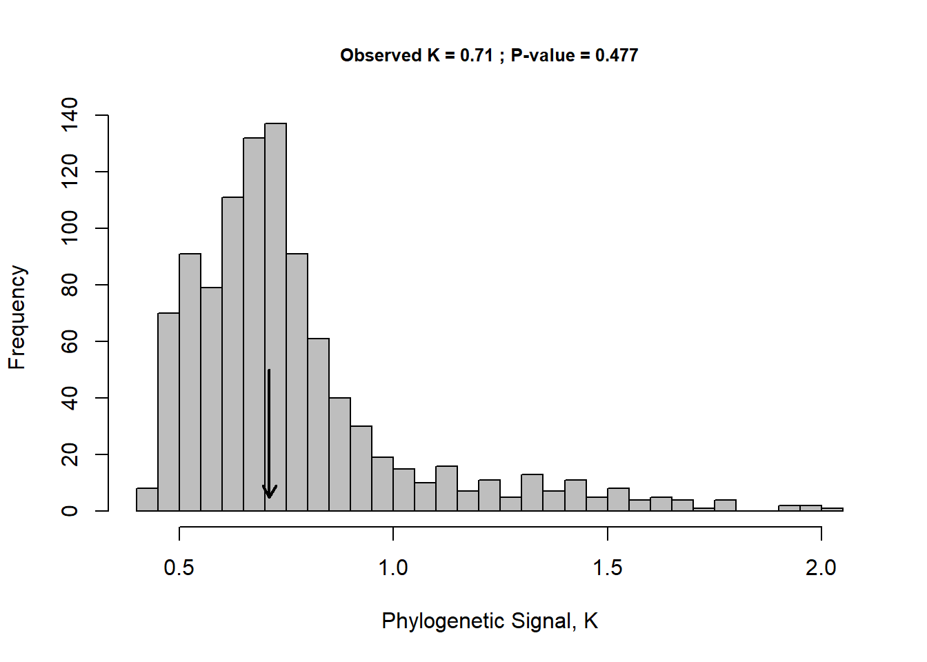
This function returns a list object containing the following which can be accessed individually using the $ operator:
physignal() Output
- \(phy.signal\): The estimate of phylogenetic signal.
- \(pvalue\): The significance level of the observed signal.
- \(random.K\): Each random K-statistic from random permutations.
- \(permutations\): The number of random permutations used in the resampling procedure.
- \(PACA\): A phylogenetically aligned component analysis, based on OLS residuals.
- \(K.by.p\): The phylogenetic signal in 1, 1:2, 1:3, …, 1:p dimensions, for the p components from PACA.
- \(call\): The matched call (input code)