6. Shape Statistics I

class: center, middle, inverse, title-slide

.title[
# 6. Shape Statistics I
]
.subtitle[
## Assessing the covariation of shape and other variables.
]
.author[
### 
]

---

### Revisiting Linear Algebra Goals

Understand why this equation is a foundational equation used in geometric morphometrics (GM)

`$$\small\mathbf{Z}=[trace[\mathbf{(Y-\overline{Y})(Y-\overline{Y})^T}]]^{-1/2}\mathbf{(Y-\overline{Y})H}$$`

Understand why this equation is a foundational equation in multivariate statistics (and burn it into your memory)

`$$\hat{\boldsymbol{\beta}}=\left ( \mathbf{\tilde{X}}^{T} \mathbf{\tilde{X}}\right )^{-1}\left ( \mathbf{\tilde{X}}^{T} \mathbf{\tilde{Z}}\right )$$`

Understand why this equation is a universal equation for describing the alignment of shape data (or any multivariate data) to an alternative set of data, covariance structure, or model

`$$\mathbf{A}^T\mathbf{Z} =\mathbf{UDV}^T$$`
---

### Revisiting Linear Algebra Goals
.pull-left[.med[

`$$\small\mathbf{Z}=[trace[\mathbf{(Y-\overline{Y})(Y-\overline{Y})^T}]]^{-1/2}\mathbf{(Y-\overline{Y})H}$$`

**Should be more obvious now, although it probably looks more obvious as `$\small\mathbf{Z}=CS^{-1}\mathbf{(Y-\overline{Y})H}$`**.

Procrustes coordinates: linear transformation of coordinate data.

----

`$$\hat{\boldsymbol{\beta}}=\left ( \mathbf{\tilde{X}}^{T} \mathbf{\tilde{X}}\right )^{-1}\left ( \mathbf{\tilde{X}}^{T} \mathbf{\tilde{Z}}\right )$$`

**Estimation of linear model coefficients for transformed data, `$\mathbf{Z}$`, which Procrustes coordinates are.**

Coefficients:  transformation of the data, based on model parameters.

----
]]

.pull-right[.med[

`$$\mathbf{A}^T\mathbf{Z} =\mathbf{UDV}^T$$`

***This one might not seem familiar.***

This is actually a basic equation.  Compare the left side to the equation before.  If `$\mathbf{A}= \mathbf{X}(\mathbf{X}^T\mathbf{X})^{-1}$`, then the the left side of the equation is the same format.

We will explore the latter two equations in detail in this lecture.
]]
---
.pull-left[
### Overview:

+ Simple Conceptual Premise
+ Principal Component Analysis
+ Partial Least Squares (PLS)
  + PLS conceptual framework
  + Hypothesis testing with RRPP
+ Alignment of data to hypothesized covariances
  + Phylogenetically Aligned Component Analysis
+ The General Linear Model (GLM)
 + Estimation with ordinary least squares
 + Estimation with generalized least squares
 + Fitted values from linear models
 + Covariance matrices
 ]
 .pull-right[
### Topics that will be covered in Shape Statistics II

+ Revisit RRPP for linear models
+ Common test statistics
+ Simple model evaluation
  + RRPP and exchangeable units under the null hypothesis
+ Multi-model evaluation
  + Nested models
    + Exchangeable units under null hypotheses
    + Types of sums of squares and cross-products
  + Non-nested models
    + Likelihood
    + AIC
+ The ability of RRPP to test better hypotheses
  + Trajectory analysis
  + Disparity analysis
+ The common thread in all statistical analyses.
    ]

---

.center[

# Part I. Simple Conceptual Premise

## Statistics is making sense of alternative data transformations

]
---

### The most basic equation

`$$\mathbf{A}^T\mathbf{Z} =\mathbf{UDV}^T$$`

Let's look at just the first part

`$$\mathbf{A}^T\mathbf{Z}$$`

What does this say to us?  First, let's adopt the tendency to see  `$\mathbf{Z}$` and assume its a transformation of data, `$\mathbf{Y}$`; i.e.,

`$$\mathbf{Z}= f(\mathbf{Y})$$`

For example, Procrustes coordinates are obtained through a transformation of coordinate data.

Second, let's develop the tendency to see `$\mathbf{A}$` and think of *.blue[association]* or *.blue[alignment]* or *.blue[adjustment]*.  A transformation of (already transformed) data either adjusts those data in some way, or aligns them to some other matrix, or maximizes some association with some other matrix.  **Thus, `$\mathbf{A}^T\mathbf{Z}$` is a transformation of data based on some idea represented by `$\mathbf{A}$`**

*Note, transformations of transformations might seem confusing, but think of basic algebra: `$ay = e(d(c(by)))$`, meaning `$a = edcb$`.*

---

### The most basic equation

`$$\mathbf{A}^T\mathbf{Z} =\mathbf{UDV}^T$$`

Although it is useful to think of `$\mathbf{A}^T\mathbf{Z}$` as a data transformation, **some caution is advised!**  Generally speaking, a ***transformation*** of data in an `$n\times p$` matrix produces an `$n\times p$` matrix.  This is possible only if `$\mathbf{A}$` is an `$n \times n$` matrix!

It is better to use the term, ***.red[association]*** or ***.red[alignment]***, as this does not convey any notion of required matrix dimensions as a result.

The next slide has some examples of what `$\mathbf{A}$` could be.
---

### Examples of `$\mathbf{A}$` matrices

.pull-left[
Let `$\mathbf{1}$` be an `$n \times 1$` vector of 1s.  Let `$\mathbf{A}^T = (\mathbf{1}^T\mathbf{1})^{-1} \mathbf{1}^T$`.  
]
.pull-right[
Then `$\mathbf{A}^T\mathbf{Z}$` **is the vector of `$p$` mean values for the `$n \times p$` matrix of data, `$\mathbf{Z}$`; i.e., `$\mathbf{A}^T\mathbf{Z} = \mathbf{\overline{z}}^T$`**
]

.pull-left[
Let `$\mathbf{1}$` be an `$n \times 1$` vector of 1s.  Let `$\mathbf{A}^T = \mathbf{1}(\mathbf{1}^T\mathbf{1})^{-1} \mathbf{1}^T$`.
]
.pull-right[
Then `$\mathbf{A}^T\mathbf{Z}$` **is an `$n \times p$` matrix where every row is `$\mathbf{\overline{z}}^T$`.**
]

.pull-left[
Let `$\mathbf{X}$` be an `$n \times 2$` matrix with one column the vector, `$\mathbf{1}$`, and the other column is `$x = CS$`, an `$n \times 1$` vector of centroid size for `$n$` specimens.  Let `$\mathbf{A}^T = (\mathbf{X}^T\mathbf{X})^{-1} \mathbf{X}^T$`.  
]
.pull-right[
Then `$\mathbf{A}^T\mathbf{Z}$` **is the matrix of regression coefficients for an analysis of allometry**
]

.remark-code[.blue[
The point is that on the left, we have `$\mathbf{A}^T$`, which is some way to align or associate our data and on the right, we have our data `$\mathbf{Z}$`.  Finding the association -- like coefficients for allometry -- might be the goal or alignment might be a step for another purpose.

Statistical analysis of shape can be thought of as a process that finds one or alternative `$\mathbf{A}^T$` solutions, decomposes them, or compares them.
]]
---

.center[
# Part II. Principal Component Analysis

## The simplest alignment: the identity matrix

]
---

### Principal component analysis (PCA)

#### How PCA is usually presented:

`$$\hat{\boldsymbol{\Sigma}} = \mathbf{V\Lambda V}^T,$$`
where

+ `$\hat{\boldsymbol{\Sigma}}$` is a residual covariance matrix (more on this soon)
+ `$\mathbf{V}$` is a rectangular matrix of eigenvectors
+ `$\mathbf{\Lambda}$` is a diagonal matrix with eigenvalues `$(\lambda)$` along the diagonal.

This presentation requires understanding how to calculate a covariance matrix (which is not a bad thing).  The following presentation might be a little easier.

---
### Principal component analysis (PCA)

#### How PCA can be presented:

`$$\mathbf{A}^T\mathbf{Z} =\mathbf{UDV}^T,$$`
where `$\mathbf{A}$` = `$\mathbf{I}_{n \times n}$`, thus

`$$\mathbf{I}^T_{n \times n} \mathbf{Z} =\mathbf{UDV}^T.$$`

+ The right singular vectors (from singular value decomposition) are the same as the eigenvectors calculated in the classic way.
+ `$\mathbf{Z}$` are data that have been .red[centered] or .red[standardized], and as such, `$\hat{\boldsymbol{\Sigma}} = (n-1)^{-1} \mathbf{Z}^T\mathbf{Z}$`.
+ `$\mathbf{D}$` is the diagonal matrix of singular values ( `$d$` ), which can be transformed to eigenvalues as `$\lambda_i = d_i^2(n-1)^{-1}$`.

***How is this easier?***  It might not seem easier yet, but when presented as `$\mathbf{A}^T\mathbf{Z}$`, one can think of how data are aligned.  In this case, they are aligned to `$\mathbf{I}_{n \times n}$`, which is like saying **independence** of alignment.

.remark-code[.blue[
In other words, PCA finds the principal vectors of variation in the data, `$\mathbf{V}$`, independent of any other association.
]]

---
### Principal component analysis (PCA)

PCA finds vectors, `$\mathbf{V}$`, from the solution,
`$$\mathbf{I}^T_{n \times n} \mathbf{Z} =\mathbf{UDV}^T.$$`
+ The relative weight of each vector (.red[*importance*]) of each vector is determined as `$\lambda_i / \sum(\lambda_i)$`, which is the same as `$d_i^2 / \sum d_i^2$`.
+ Each PC (vectors of `$\mathbf{V}$`) is a linear combination of the variables in `$\mathbf{Z}$`, called .red[*loadings*].
+ Projection of the centered or standardized data onto the PCs is done as
`$$\mathbf{P} = \mathbf{ZV},$$` meaning `$\mathbf{P}$` is a matrix of PC scores.
+ The number of vectors in `$\mathbf{V}$` is at most `$\min(p, n-1)$`, but can be fewer because of redundancies in the data.  ***This is always the case with shape data, because of GPA!***  
+ An easier way to determine the number of dimensions is to find the cases where `$\lambda_i > tol$`, where `$tol$` is a value near 0, such that any value below it can be considered 0.

---

### Principal component analysis (PCA)

#### Example with `plethodon` data in `geomorph`
.med[

``` r
data(plethodon)
GPA <- gpagen(plethodon$land, print.progress = FALSE)
* PCA <- gm.prcomp(GPA$coords) 
```

Let's look at the `$\mathbf{V}$` matrix (PC vector loadings) for the first 5 vectors.  Recall from the lecture on linear algebra, `$\mathbf{V}$` is the same as a *rotation* matrix.

``` r
PCA$rot[, 1:5]
```

<div class="datatables html-widget html-fill-item" id="htmlwidget-22393721229cfd213307" style="width:100%;height:auto;"></div>
<script type="application/json" data-for="htmlwidget-22393721229cfd213307">{"x":{"filter":"none","vertical":false,"fillContainer":false,"data":[["1.X","1.Y","2.X","2.Y","3.X","3.Y","4.X","4.Y","5.X","5.Y","6.X","6.Y","7.X","7.Y","8.X","8.Y","9.X","9.Y","10.X","10.Y","11.X","11.Y","12.X","12.Y"],[-0.18519,0.05405,-0.25751,0.12104,0.24555,0.08671,0.01913,0.01574,0.03013,-0.06,0.03942,-0.07298,-0.03292,-0.15883,-0.07436,-0.02267,-0.1294,0.14563,-0.14615,0.04686,0.78142,-0.05272,-0.29012,-0.10285],[0.44578,0.26015,0.14487,0.35368,0.06079,0.15116,-0.00471,-0.10675,-0.04475,-0.10706,-0.02427,-0.16916,-0.14499,-0.08201,-0.0491,-0.01583,0.0163,0.10257,0.07706,0.13217,-0.18989,0.04808,-0.28709,-0.56701],[0.22986,-0.08275,0.21506,0.10056,0.32681,0.00228,-0.20322,0.35931,-0.19877,0.15439,-0.17122,0.009809999999999999,-0.21542,-0.18189,0.06254,-0.16576,0.18179,-0.23899,0.07886,-0.13614,0.01087,-0.20317,-0.31717,0.38235],[-0.26247,0.11272,-0.01087,0.46841,0.47658,-0.04908,-0.11434,-0.00444,-0.05717,0.12899,0.1062,0.0582,0.08944000000000001,0.01527,-0.1435,-0.17252,-0.17443,-0.1315,-0.16718,-0.21664,-0.17314,-0.06654,0.43089,-0.14288],[-0.16719,0.22104,0.02176,-0.25447,0.44786,0.02916,-0.0437,-0.44113,-0.16144,-0.22846,-0.05394,0.14802,0.0188,0.27939,-0.08595,0.08477999999999999,0.38216,0.11626,-0.05794,0.12139,-0.12552,-0.17414,-0.1749,0.09816]],"container":"<table class=\"display\">\n  <thead>\n    <tr>\n      <th> <\/th>\n      <th>Comp1<\/th>\n      <th>Comp2<\/th>\n      <th>Comp3<\/th>\n      <th>Comp4<\/th>\n      <th>Comp5<\/th>\n    <\/tr>\n  <\/thead>\n<\/table>","options":{"pageLength":3,"columnDefs":[{"className":"dt-right","targets":[1,2,3,4,5]},{"orderable":false,"targets":0},{"name":" ","targets":0},{"name":"Comp1","targets":1},{"name":"Comp2","targets":2},{"name":"Comp3","targets":3},{"name":"Comp4","targets":4},{"name":"Comp5","targets":5}],"order":[],"autoWidth":false,"orderClasses":false,"lengthMenu":[3,10,25,50,100]}},"evals":[],"jsHooks":[]}</script>
]

---
.pull-left[
### Principal component analysis (PCA)

#### Example with `plethodon` data in `geomorph`

The .blue[`gm.prcomp`] function performs projection, and returns PC scores as `$x`.  These can be extracted and plotted, or one can use the generic plot function.

We can ascertain that the first axis explains almost 37% of the shape variation and the second axis, about 31% of the shape variation.  Different groups (as differentiated by symbol and color) are in different locations of the PC space, suggesting some shape differences.
]
.pull-right[.med[

``` r
plot(PCA, 
     pch = 15 + as.numeric(plethodon$site), 
     col = plethodon$species, cex = 2)
```

![](06-ShapeStatistics1_files/figure-html/unnamed-chunk-4-1.png)
]]
---

### Principal component analysis (PCA)

#### Comments

+ PCA is the most basic way to look at a high-dimensional data space in discernible dimensions.
+ Alignment of data to its inherent, principal axes.
+ A rigid rotation of the data space (orthogonal projection)
+ The distances among observed shapes in all PC dimensions is the same as the distances in original dimensions, so long as `$\sum\lambda_i = trace(\hat{\boldsymbol{\Sigma}})$`.  In other words, the diagonals of `$(n-1)^{-1}\mathbf{ZZ}^T$` and `$\mathbf{PP}^T$` have the same sum.
+ .remark-code[.red[Some sources discuss PCA performed on either covariance or correlation matrices.  **This is unnecessary.**  If `$\mathbf{Z}$` is a matrix of centered data, then `$\hat{\boldsymbol{\Sigma}}$` is a covariance matrix; if `$\mathbf{Z}$` is a matrix of standardized data, then `$\hat{\boldsymbol{\Sigma}}$` is a correlation matrix.  Performing PCA on a correlation matrix is simply making the *a priori* decision to standardize data `$^1$`.
]]

.footnote[1. Data centering and standardization are discussed in the appendix for these lectures.]

---

.center[
# Part III. Partial Least Squares

## Alignment of shape data to other data

]
---

### Partial Least Squares

.blue[**Partial least squares (PLS)**] is the basis for finding the association between two matrices, taking the form of
`$$\mathbf{A}^T\mathbf{Z} =\mathbf{UDV}^T,$$`

where `$\mathbf{A}$` is an alternative set of data, like `$\mathbf{Z}$`.  Therefore, we can update the equation above to be:

`$$\mathbf{Z}_1^T\mathbf{Z}_2 =\mathbf{UDV}^T,$$`
where `$\mathbf{Z}_1$` and `$\mathbf{Z}_2$` are both sets of data that have been .red[centered] or .red[standardized].

PLS is the basis for various statistical alternatives, including correlation, linear regression, and structural equation modelling.

PLS is a method that finds the maximum covariation between data sets, and allows one to consider if and to what extent shape covaries with other data.

---

### Partial Least Squares

If we let `$\mathbf{Z}_2$` be a set of shape data, `$\mathbf{Z}_1$` can be the alternative data with which shape data putatively covary.  Examples of alternative data might include:

+ Other shape data (from different structures)
+ Specimen size (allometry)
+ Performance data (linking form and function)
+ Life history data (co-evolution of fitness-related traits?)

Additionally, shape data might be split into subsets (**modules**) to examine how **integrated** the separate morphological modules are.  We defer this more in-depth consideration to the lecture on **Integration and Modularity**.

---

### Partial Least Squares

`$$\mathbf{Z}_1^T\mathbf{Z}_2 =\mathbf{UDV}^T,$$`
.pull-left[
The singular value decomposition (SVD) finds two sets of vectors.

+ The ***.blue[left]*** vectors, `$\mathbf{U}$` are the set of latent vectors that maximize the covariation of `$\mathbf{Z}_1$` to  `$\mathbf{Z}_2$`
+ The ***.blue[right]*** vectors, `$\mathbf{V}$` are the set of latent vectors that maximize the covariation of `$\mathbf{Z}_2$` to  `$\mathbf{Z}_1$`
+ The diagonal matrix, `$\mathbf{D}$` contains the ***.blue[singular values]*** that are weights expressing the strength of covariation between vector pairs (e.g., between `$\mathbf{u}_1$` and `$\mathbf{v}_1$` or between `$\mathbf{u}_2$` and `$\mathbf{v}_2$`).]

.pull-right[
***.blue[PLS scores]*** can be calculated as

`$$\mathbf{P}_1 = \mathbf{Z}_1\mathbf{U}$$`
`$$\mathbf{P}_2 = \mathbf{Z}_2\mathbf{V}$$`

These scores represent a shear of each data space, constrained by the other.  This is awkward for plotting and does not offer any easy interpretations for how shape changes in the separate data spaces.

Rather, Rohlf and Corti (2000) recommended using the correlation between `$\mathbf{p}_{1_{1}}$` and `$\mathbf{p}_{2_{1}}$`, which can be visualized with a scatter-plot.]

.footnote[Rohlf & Corti. (2000). *Systematic Biology.*]

---

### Partial Least Squares, the GM paradigm

It is worth reiterating that PLS is a SVD of `$\mathbf{Z}_1^T\mathbf{Z}_2$`, and that multiple statistical methods could be approached with the result.

However, the typical ***GM paradigm*** via PLS is to do the following:

1. Perform `$\mathbf{Z}_1^T\mathbf{Z}_2 =\mathbf{UDV}^T$`.
2. Calculate `$\mathbf{P}_1 = \mathbf{Z}_1\mathbf{U}$` and `$\mathbf{P}_2 = \mathbf{Z}_2\mathbf{V}$`, retaining just the first PLS scores for each set, `$\mathbf{p}_{1_{1}}$` and `$\mathbf{p}_{2_{1}}$`
3. Obtain the correlation coefficient between the scores, `$r_{PLS}$`. `$^1$`
4. Make a plot of `$\mathbf{p}_{2_{1}}$` versus `$\mathbf{p}_{1_{1}}$`
5. Assess how shape changes along `$\mathbf{p}_{2_{1}}$`, and possibly `$\mathbf{p}_{1_{1}}$`, if `$\mathbf{Z}_1$` is also a set of shape data.
6. Perform a statistical test on `$r_{PLS}$`. `$^2$`

.footnote[1. Rohlf and Corti (2000) demonstrated that a correlation coefficient could be obtained via the singular values of the SVD, provided data were standardized.  Finding the correlation coefficient of PLS scores is a simpler heuristic.

2. A permutation test is used for statistical evaluation.  More on this a bit later.]
---
### Partial Least Squares, the GM paradigm

#### Statistical Comment

.pull-left[
PLS is generally presented as partitioning of a covariance matrix, but this is not fully necessary.

If we concatenate our data, `$\mathbf{Z} = \mathbf{Z}_1 | \mathbf{Z}_2$`, then a covariance matrix found as `$\hat{\boldsymbol{\Sigma}} = (n-1)^{-1}\mathbf{Z}^T\mathbf{Z}$` has the following form.

![](06-ShapeStatistics1_files/figure-html/unnamed-chunk-5-1.png)
]

.pull-right[
+ The upper-left (darkest) block is the covariance matrix for `$\mathbf{Z}_1$`
+ The lower-right (dark) block is the covariance matrix for `$\mathbf{Z}_2$`
+ The other (light) blocks are the covariances between the covariance blocks, and are equal via a transpose.
+ The upper block is the same as `$(n-1)^{-1}\mathbf{Z}_1^T\mathbf{Z}_2$`, which has the same singular vectors as `$\mathbf{Z}_1^T\mathbf{Z}_2$`; singular values that differ in scale by `$(n-1)$`.
]
---

### Partial Least Squares, the GM paradigm

#### Statistical Comment

.pull-left[
PLS is generally presented as partitioning of a covariance matrix, but this is not fully necessary.

+ **.blue[PLS is generally referred to as two-block PLS based on this original presentation by Rohlf and Corti (2000)] .red[but there is no need to calculate a covariance matrix and partition it]**

+ Finding `$\mathbf{Z}_1^T\mathbf{Z}_2$` is sufficient.
]

---

### Partial Least Squares, Example

Before getting into a statistical test, let's look at the steps of the **.blue[GM PLS paradigm]** with an example

+ Example from Adams, D. C., and F. J. Rohlf. 2000. Ecological character displacement in Plethodon: biomechanical differences found from a geometric morphometric study. Proceedings of the National Academy of Sciences, U.S.A. 97:4106-4111

+ These data contain head shape data from 13 landmarks for plethodontid salamanders, plus gut content data (square-root transformed frequencies of 16 taxonomic groups).

.center[
<img src="LectureData/06.shapestatistics1/plethExample1.png" width="90%" />
]
---

### Partial Least Squares, Example

Before getting into a statistical test, let's look at the steps of the **.blue[GM PLS paradigm]** with an example

+ These data contain head shape data from 13 landmarks for plethodontid salamanders, plus gut content data (square-root transformed frequencies of 16 taxonomic groups).

**First, data analysis set up.**

``` r
data(plethShapeFood) 
GPA <- gpagen(plethShapeFood$land, print.progress = FALSE) 
Z2 <- GPA$coords
Z1 <- plethShapeFood$food
rownames(Z1) <- dimnames(Z2)[[3]]
* PLS <- two.b.pls(Z1, Z2, print.progress = FALSE)
```

---

### Partial Least Squares, Example

**Second, left and right singular vectors.**  Only the first few are shown.

.pull-left[.small[

``` r
PLS$left.pls.vectors[, 1:3]
```

```
##                 [,1]         [,2]        [,3]
## oligoch   0.09004086 -0.003112899  0.10080188
## gastrop  -0.01806988  0.550910355 -0.34547832
## isopoda   0.04248161 -0.341360115  0.01758372
## diplop    0.05513422 -0.382587566  0.20527963
## chilop    0.09336132 -0.037443265  0.04266139
## acar     -0.50752475 -0.019441095  0.41786654
## araneida  0.25374179  0.046295602  0.40983773
## chelon   -0.11208684  0.285524589  0.47666133
## coleopt   0.49499065 -0.224817353 -0.03268055
## collemb  -0.39472156 -0.072040810  0.09579918
## diptera   0.16588149  0.046529118  0.23630937
## hymen     0.36492582  0.498143789  0.27865952
## isopt    -0.11941724  0.133602846 -0.25262551
## orthopt   0.12637425 -0.040163997 -0.02415219
## larvae    0.21581022 -0.077047426  0.13298564
## eggs     -0.07184867  0.129214952  0.17493561
```
]]
.pull-right[.small[

``` r
PLS$right.pls.vectors[, 1:3]
```

```
##             [,1]         [,2]         [,3]
## 1.X   0.13133953 -0.016017800 -0.027231576
## 1.Y   0.14787439 -0.064700347  0.002158334
## 2.X   0.18997240  0.085495097  0.016186956
## 2.Y   0.21071931  0.041299482  0.160306629
## 3.X  -0.10497337  0.278032904  0.217025988
## 3.Y   0.01823770  0.011813496  0.023272786
## 4.X   0.02175516 -0.014456289 -0.236713711
## 4.Y  -0.29628475  0.050082411 -0.049278170
## 5.X  -0.03246685  0.057861386 -0.169413647
## 5.Y  -0.30786568 -0.049237233 -0.041987632
## 6.X   0.04097434  0.307022495  0.528304865
## 6.Y   0.26835518 -0.281134207  0.261101618
## 7.X   0.08484467  0.072600350 -0.258164600
## 7.Y   0.10011120 -0.351750512  0.199695532
## 8.X   0.24257232 -0.199231902 -0.319392449
## 8.Y  -0.27613187 -0.102491653 -0.029819586
## 9.X  -0.52125417 -0.365570595  0.248722170
## 9.Y  -0.29871448  0.283290297 -0.160260576
## 10.X -0.01313886 -0.341927800 -0.085658889
## 10.Y  0.13148260  0.225262939  0.076937140
## 11.X -0.02765115 -0.184773252 -0.070110492
## 11.Y  0.12231665  0.088280534  0.029395633
## 12.X -0.07705921  0.329160469 -0.015287345
## 12.Y -0.04872696  0.124990718 -0.363320979
## 13.X  0.06508520 -0.008195063  0.171732729
## 13.Y  0.22862671  0.024294075 -0.108200731
```
]]

---

### Partial Least Squares, Example

**Third, projected PLS scores.**  *Note that scores are called X- and Y-scores, just to be consistent with axes in a scatter plot.*  There as many vectors of scores as there are vectors, `$\min(p_1, p_2)$`.  Only the first vector scores are shown.

.pull-left[.small[

``` r
PLS$XScores[,1]
```

```
##           1           2           3           4           5           6 
##  0.40971817  1.23459068  0.82354660  2.25474965  1.16861235  1.54211178 
##           7           8           9          10          11          12 
##  2.40814581  1.38648891  1.47572148  1.15145628  1.82488211  2.00281727 
##          13          14          15          16          17          18 
##  1.70842839  0.78350966  2.35656647  1.97025758  1.32711128  2.45518339 
##          19          20          21          22          23          24 
##  1.13194734  1.19586428  1.57987261  0.56092041  1.69775574 -0.51771460 
##          25          26          27          28          29          30 
##  1.78944625  0.41542579  1.47244700  1.96359871  0.82169641  1.82440476 
##          31          32          33          34          35          36 
##  1.18331357  1.20800520  1.45332637  0.46107422  0.43077595  0.44272421 
##          37          38          39          40          41          42 
##  0.12521551  0.08737129 -1.49198346 -1.08751911 -1.65355327  0.43789394 
##          43          44          45          46          47          48 
## -0.78538045 -1.31611152 -1.92185107 -2.38907027 -3.86537030 -0.69053902 
##          49          50          51          52          53          54 
## -3.54536310 -2.36767049 -1.73181625 -1.92996848 -2.48100918 -0.53394348 
##          55          56          57          58          59          60 
## -0.97138038 -1.76287413 -1.47704837 -1.47140411 -1.37297335 -2.35545959 
##          61          62          63          64          65          66 
## -0.72666303 -1.19599325 -1.85655314 -2.02790901 -0.87425893 -0.57034773 
##          67          68          69 
## -2.00072299 -0.41353290 -1.18099243
```
]]
.pull-right[.small[

``` r
PLS$YScores[,1]
```

```
##             1             2             3             4             5 
## -0.0084886128  0.0145782821  0.0715922727  0.0446059322  0.0488893887 
##             6             7             8             9            10 
##  0.0463305289 -0.0013728175  0.0161337492  0.0439645798  0.0225700350 
##            11            12            13            14            15 
##  0.0481547796  0.0235046767  0.0685178310  0.0468964791  0.0661361442 
##            16            17            18            19            20 
## -0.0200428036  0.0059616234  0.0269170135  0.0450323403  0.0815084485 
##            21            22            23            24            25 
##  0.0371587080  0.0665039743  0.0116523749  0.0541575000  0.0207313601 
##            26            27            28            29            30 
## -0.0190376464  0.0424146827  0.0243060884  0.0294380511  0.0725344576 
##            31            32            33            34            35 
## -0.0131989687  0.0724950592  0.0577080367  0.0213928113  0.0666798204 
##            36            37            38            39            40 
##  0.0229458025  0.0027351589  0.0078255518  0.0048385137 -0.0304243293 
##            41            42            43            44            45 
## -0.0284378257  0.0266160579 -0.0457595930 -0.0350006883  0.0003095332 
##            46            47            48            49            50 
## -0.0694581548 -0.0845256482 -0.0327183823 -0.1226806712 -0.0584908355 
##            51            52            53            54            55 
## -0.0123083358 -0.0799193543 -0.0773655677 -0.0498207761  0.0543905645 
##            56            57            58            59            60 
## -0.0331319321 -0.0569223733 -0.0496096225 -0.0607295822 -0.0232294676 
##            61            62            63            64            65 
##  0.0038645939 -0.0193132260 -0.0225186430 -0.0548283429 -0.0954926995 
##            66            67            68            69 
## -0.0576659593 -0.0476004219 -0.0643488192 -0.0475507053
```
]]

---

### Partial Least Squares, Example

**Fourth, scatter plot of scores and `$r_{PLS}$`.**

.pull-left[.med[

``` r
PLS
```

```
## 
## Call:
## two.b.pls(A1 = Z1, A2 = Z2, print.progress = FALSE) 
## 
## 
## 
## r-PLS: 0.759
## 
## Effect Size (Z): 3.9379
## 
## P-value: 0.001
## 
## Based on 1000 random permutations
```

*Ignore `$P$`-value and `$Z$`-score for now.*
]]
.pull-right[.small[

``` r
plot(PLS, pch = 16)
```

![](06-ShapeStatistics1_files/figure-html/unnamed-chunk-13-1.png)
]]

---

### Partial Least Squares, Example

These data contain head shape data from 13 landmarks for plethodontid salamanders, plus gut content data (square-root transformed frequencies of 16 taxonomic groups).

**Evaluation (gut content values):** It is clear that there is an association between the shape of salamander heads and what they eat.  We can understand the association by looking at first vector loadings for food along with the scatter plot.

.pull-left[.med[

``` r
PLS$left.pls.vectors[, 1]
```

```
##     oligoch     gastrop     isopoda      diplop      chilop        acar 
##  0.09004086 -0.01806988  0.04248161  0.05513422  0.09336132 -0.50752475 
##    araneida      chelon     coleopt     collemb     diptera       hymen 
##  0.25374179 -0.11208684  0.49499065 -0.39472156  0.16588149  0.36492582 
##       isopt     orthopt      larvae        eggs 
## -0.11941724  0.12637425  0.21581022 -0.07184867
```

*Look at the largest loadings, whether negative or positive, and associate this with the axis in the plot.*

]]
.pull-right[.small[

``` r
plot(PLS, pch = 16)
```

![](06-ShapeStatistics1_files/figure-html/unnamed-chunk-15-1.png)
]]

---

**Evaluation (head shape):** It is clear that there is an association between the shape of salamander heads and what they eat.  We can understand the association by looking at head shape change at vector extremes.

.pull-left[.small[
***Could use*** `picknplot.shape` ***instead of this code below.***

``` r
preds <- shape.predictor(A = PLS$A2, 
                         x = PLS$YScores[, 1],
                         Intercept = FALSE,
                         method = "PLS",
                         yAxis1min = min(PLS$YScores[, 1]),
                         yAxis1max = max(PLS$YScores[, 1]))

Ref <- mshape(PLS$A2)

par(mfrow = c(1, 2))
plotRefToTarget(Ref, preds$yAxis1min)
title("Shape at min PLS 1")
plotRefToTarget(Ref, preds$yAxis1max)
title("Shape at max PLS 1")
```

![](06-ShapeStatistics1_files/figure-html/unnamed-chunk-16-1.png)

]]
.pull-right[.small[

``` r
plot(PLS, pch = 16)
```

![](06-ShapeStatistics1_files/figure-html/unnamed-chunk-17-1.png)

``` r
PLS$left.pls.vectors[, 1]
```

---

### Partial Least Squares, a few other examples

**Shape allometry**

The covariation between shape and size; i.e., how shape changes as organisms grow or develop.
---

### Partial Least Squares, a few other examples

.pull-left[.med[

**Shape allometry**

`$\mathbf{Z}_1$` is a vector of the log of centroid size

``` r
Z1 <- log(GPA$Csize)
PLS <- two.b.pls(Z1, Z2, print.progress = FALSE)
PLS
```

```
## 
## Call:
## two.b.pls(A1 = Z1, A2 = Z2, print.progress = FALSE) 
## 
## 
## 
## r-PLS: 0.826
## 
## Effect Size (Z): 5.5569
## 
## P-value: 0.001
## 
## Based on 1000 random permutations
```
]]
.pull-right[.small[

``` r
plot(PLS, pch = 16)
```

![](06-ShapeStatistics1_files/figure-html/unnamed-chunk-19-1.png)

Notice this:

``` r
(log(GPA$Csize) - mean(log(GPA$Csize)))[1:5]
```

```
##           1           2           3           4           5 
##  0.02675961 -0.05866555  0.23522474  0.16773141 -0.06493891
```

``` r
PLS$XScores[1:5, 1]
```

```
##           1           2           3           4           5 
## -0.02675961  0.05866555 -0.23522474 -0.16773141  0.06493891
```
]]

---

### Partial Least Squares, a few other examples

**Module shape covariation**

The strength of covariation among sub-configurations of a landmark configuration, which are hypothetical genetic/developmental modules.

---

### Partial Least Squares, a few other examples

.pull-left[.med[

**Module shape covariation**

``` r
Z1 <- GPA$coords[1:5, , ] # Five landmarks of jaw
Z2 <- GPA$coords[6:13, , ] # 8 landmarks of cranium
PLS <- two.b.pls(Z1, Z2, print.progress = FALSE)
PLS
```

```
## 
## Call:
## two.b.pls(A1 = Z1, A2 = Z2, print.progress = FALSE) 
## 
## 
## 
## r-PLS: 0.912
## 
## Effect Size (Z): 6.8648
## 
## P-value: 0.001
## 
## Based on 1000 random permutations
```
]]

.pull-right[.small[

``` r
plot(PLS, pch = 16, asp = 1)
```

![](06-ShapeStatistics1_files/figure-html/unnamed-chunk-22-1.png)
]]

---

### Partial Least Squares, a few other examples

.pull-left[.small[

**Module shape covariation**

``` r
plot(PLS, pch = 16, asp = 1)
```

**Jaw shapes at the extremes**

``` r
predsJ <- shape.predictor(A = PLS$A1, 
                         x = PLS$XScores[, 1],
                         Intercept = FALSE,
                         method = "PLS",
                         xAxis1min = min(PLS$XScores[, 1]),
                         xAxis1max = max(PLS$XScores[, 1]))

RefJ <- mshape(PLS$A1)
```

**Neurocranium shapes at the extremes**

``` r
predsN <- shape.predictor(A = PLS$A2, 
                         x = PLS$YScores[, 1],
                         Intercept = FALSE,
                         method = "PLS",
                         yAxis1min = min(PLS$YScores[, 1]),
                         yAxis1max = max(PLS$YScores[, 1]))

RefN <- mshape(PLS$A2)
```
]]

.pull-right[.small[

**Transformation grids**

``` r
par(mfrow = c(2, 2))
plotRefToTarget(RefN, predsN$yAxis1min)
title("Neuro shape at min PLS 1")
plotRefToTarget(RefN, predsN$yAxis1max)
title("Neuro shape at max PLS 1")
plotRefToTarget(RefJ, predsJ$xAxis1min)
title("Jaw shape at min PLS 1")
plotRefToTarget(RefJ, predsJ$xAxis1max)
title("Jaw shape at max PLS 1")
```
]]

---

### Partial Least Squares, a few other examples

.pull-left[

![](06-ShapeStatistics1_files/figure-html/unnamed-chunk-27-1.png)
]

.pull-right[

![](06-ShapeStatistics1_files/figure-html/unnamed-chunk-28-1.png)
]

---

### Partial Least Squares, a partial summary

+ PLS obtains a matrix cross-product and performs SVD
+ Left vectors scores are projections of `$\mathbf{Z}_1$` on vectors that maximize covariation between `$\mathbf{Z}_1$` and `$\mathbf{Z}_2$`
+ Right vectors scores are projections of `$\mathbf{Z}_2$` on vectors that maximize covariation between `$\mathbf{Z}_1$` and `$\mathbf{Z}_2$`
+ The correlation between these scores in an easy way to appreciate the amount of covariation between matrices, at least in the principal axes that maximize their covariation.
+ .blue[But what about these inferential statistics?]

---

### Hypothesis testing for matrix covariation

A null hypothesis test is one that tests the independence (no covariation) between two matrices.  Null and alternative hypotheses can be thought of as this series of dichotomies (becoming increasingly more technical):

|Null hypothesis | Alternative hypothesis|
|----|----|
|Two matrices are independent|Two matrices are associated|
|The singular values of a matrix cross-product are rather uniform in distribution|The singular values of a matrix cross-product are skewed, such that the first or first few are much larger than the last|
|.red[The correlation between left and right vectors scores is no different than what can be expected by chance, from random combinations of vectors]|.blue[The correlation between left and right vectors scores is larger than what can be expected by chance, from random combinations of vectors.]

Every test of a null hypothesis must have a process of generating randomness under the null hypothesis.  For the case of matrix covariation, the null process is **randomization of the pairs of vectors** among the observations.  This occurs by randomizing the row vectors of either `$\mathbf{Z}_1$` or `$\mathbf{Z}_2$`.

Because `$\mathbf{Z}_1$` and `$\mathbf{Z}_2$` are both centered or standardized, they are **residuals** (of the mean).  Randomizing residuals in a permutation procedure (**.blue[RRPP]**) is used with shape data to generate test-statistic sampling distributions.
---

### Randomization of residuals in a permutation procedure (RRPP) for `$r_{PLS}$`

.pull-left[
**Algorithm:**
1. Calculate `$r_{PLS}$` `$^1$`
2. In thousands of permutations:

+ Find `$\mathbf{Z}_1^*$` by shuffling the rows of `$\mathbf{Z}_1$`
  + Perform SVD on `$(\mathbf{Z}_1^*)^T\mathbf{Z}_2$`
  + Calculate PLS scores and calculate `$r_{PLS}^*$`
  
3. Calculate the percentile of `$r_{PLS}$`: the `$P$`-value
4. Normalize the distribution as `$\theta = f(r)$`; e.g., `$^2$`
5. Find `$Z$` as the `$\theta$` mapped for `$r_{PLS}$`.
]

.pull-right[

**The `$P$`-value is a statistic that allows one to reject the null hypothesis, if below the level of significance, `$\alpha$` (usually 0.05).**

**The `$Z$`-score is an effect size that can be compared to effect sizes from other samples.  Whereas `$r_{PLS}$` is influenced by sample size and variable number, and difficult to interpret, `$Z$` is unambiguous. `$^3$`**
]

.pull-right[.footnote[
1. Could also use first singular value or sum of first few singular values, if considering multiple axes. 
2. Using, e.g., a Box-Cox transformation; 
3. Adams & Collyer. (2016). *Evolution*.
]]

---

### Examples again, paying attention to inferential statistics

.pull-left[.small[

``` r
GPA <- gpagen(plethShapeFood$land, print.progress = FALSE) 
food <- plethShapeFood$food
rownames(food) <- names(GPA$Csize)
PLSfood <- two.b.pls(food, GPA$coords, 
                  print.progress = FALSE, iter = 9999)
PLSallometry <- two.b.pls(log(GPA$Csize), GPA$coords, 
                  print.progress = FALSE, iter = 9999)
PLSintegration <- two.b.pls(GPA$coords[1:5,, ], GPA$coords[8:13,,], 
                  print.progress = FALSE, iter = 9999)
summary(PLSfood)
```

```
## 
## Call:
## two.b.pls(A1 = food, A2 = GPA$coords, iter = 9999, print.progress = FALSE) 
## 
## 
## 
## r-PLS: 0.7591
## 
## Effect Size (Z): 4.31522
## 
## P-value: 1e-04
## 
## Based on 10000 random permutations
```
]]

.pull-right[.small[

``` r
summary(PLSallometry)
```

```
## 
## Call:
## two.b.pls(A1 = log(GPA$Csize), A2 = GPA$coords, iter = 9999,  
##     print.progress = FALSE) 
## 
## 
## 
## r-PLS: 0.8262
## 
## Effect Size (Z): 5.5256
## 
## P-value: 1e-04
## 
## Based on 10000 random permutations
```

``` r
summary(PLSintegration)
```

```
## 
## Call:
## two.b.pls(A1 = GPA$coords[1:5, , ], A2 = GPA$coords[8:13, , ],  
##     iter = 9999, print.progress = FALSE) 
## 
## 
## 
## r-PLS: 0.8979
## 
## Effect Size (Z): 5.93647
## 
## P-value: 1e-04
## 
## Based on 10000 random permutations
```
]]

---
### Examples again, paying attention to inferential statistics

We can also perform *two-sample Z-tests* to see if any of these effect sizes differ.

.pull-left[.med[

``` r
compare.pls(PLSfood, PLSallometry, PLSintegration)
```

```
## 
## Effect sizes
## 
##        PLSfood   PLSallometry PLSintegration 
##       4.315216       5.525605       5.936474 
## 
## Effect sizes for pairwise differences in PLS effect size
## 
##                 PLSfood PLSallometry PLSintegration
## PLSfood        0.000000    2.3754635      3.0941152
## PLSallometry   2.375463    0.0000000      0.7977631
## PLSintegration 3.094115    0.7977631      0.0000000
## 
## P-values
## 
##                    PLSfood PLSallometry PLSintegration
## PLSfood        1.000000000   0.01752693    0.001974008
## PLSallometry   0.017526928   1.00000000    0.425007955
## PLSintegration 0.001974008   0.42500796    1.000000000
```
]]

.pull-right[
**Thus, covariation between shape and prey acquired is significant but the effect size is significantly smaller that head-jaw shape integration or shape allometry.**

Note: two-sample `$Z$` statistic is found as `$Z_{12} = \frac{| (\theta_1 - \mu_1) - (\theta_2 - \mu_2) | }{\sqrt{\sigma_1^2 +\sigma_2^2}}$`, where `$\mu$` and `$\sigma$` are the mean and standard deviation of an RRPP sampling distribution for `$\theta$`, the normalized value of `$r_{PLS}$`.  The `$P$`-value is estimated from integration of a standard normal probability density function.
]

---

### Hypothesis testing for matrix covariation, summary and comments

+ Regardless of inferential statistical methods, it is assumed that a null process generates random variation, given a set of conditions.
  + Parametric statistics (not discussed here) use probability density or mass functions ***as a proxy*** for the *distribution of all possible random outcomes* of a null process, provided assumptions are met.
  + RRPP performs a subset of random permutations ***as a proxy*** for the *distribution of all possible random outcomes* of a null process.
+ Why RRPP rather than parametric statistics?
  + produces commensurate distributions with parametric density functions, under appropriate conditions. `$^1$`
  + No parametric proxy? RRPP can still be used.
  + Fast computers.
+ **.blue[For PLS analyses, RRPP = randomizing the row vectors of only one set of data (sufficient to make random pairs of vectors).  Independent data?  Random] `$r_{PLS}$` .blue[values consistently as large as the observed value.  Data sets covary?] `$r_{PLS}$` .blue[will be rare (in a large way).]**
+ **.green[Two-sample] `$Z$`.green[-tests can be performed to compare the effect sizes from different PLS analyses.]**

.footnote[1. Several papers by Adams and Collyer have illustrated this.  Most recently: Adams & Collyer. (2022). *Evolution*.
]

---

.center[
# Part IV. Alignment of data to a matrix of hypothesized covariances among observations

## Although a general application, there is one established method for GM data: Phylogenetically aligned component analysis (PACA)

]
---

### Alignment of data to a hypothesized covariance matrix

An hypothesized covariance matrix is different than a residual covariance matrix.  It is a matrix of expected covariances because on an inherent relatedness among observations (the observations are not independent)

Examples include:

+ A covariance matrix for spatial auto-correlation based on a particular spatial model
+ A covariance matrix for temporal auto-correlation (repeated measures analysis) based on a particular model for the frequency and intervals of measurement
+ ** A covariance matrix for evolutionary correlations based on a model of evolutionary divergence.**

.blue[Because GM analyses tend to focus on comparative data, we present this with phylogenetic covariances, but the concepts can be applied to other data types.]

`$$\mathbf{A}^T\mathbf{Z} = \mathbf{UDV}^T$$`

Let `$\mathbf{A} = \boldsymbol{\Omega}$`, where `$\boldsymbol{\Omega}$` is an `$N \times N$` matrix of phylogenetic covariances, assuming a Brownian motion model of evolutionary divergence, corresponding to the `$N \times p$` matrix of centered or standardized data, `$\mathbf{Z}$`.  Then,

`$$\boldsymbol{\Omega}^T\mathbf{Z} = \mathbf{UDV}^T$$`

is an analysis that finds phylogenetically aligned components of the data (most phylogenetic signal in the first few components).

---

### Phylogenetically aligned component analysis (PACA) `$^1$`

`$$\boldsymbol{\Omega}^T\mathbf{Z} = \mathbf{UDV}^T$$`
+ `$\mathbf{Z}$` is an `$N \times p$` matrix of centered or standardized data.  (We use `$N$` rather than `$n$` because these are the `$N$` taxonomic observations in the phylogenetic tree considered, rather than `$n$` observations sampled from a population of `$N$` data.)
+ `$\boldsymbol{\Omega}$` is an `$N \times N$` covariance matrix, based on a phylogenetic tree, with the depth of an *ultrametric phylogenetic tree* (consistent sum of branch lengths from root to tip) and the off-diagonal elements are phylogenetic covariances (shared branch lengths from root to common ancestors, which can be 0 for taxa in different clades)
+ **See next slide for illustration.**

.footnote[1. Collyer & Adams. (2021). *Methods in Ecology and Evolution*.]
---

### Phylogenetically aligned component analysis (PACA) `$^1$`

.pull-left[
**Tree**

```
## Loading required package: ape
```

```
## Loading required package: maps
```

![](06-ShapeStatistics1_files/figure-html/unnamed-chunk-32-1.png)
]

.pull-right[
**Covariance matrix**

```
##       t3    t4    t1    t2
## t3 0.531 0.490 0.000 0.000
## t4 0.490 0.531 0.000 0.000
## t1 0.000 0.000 0.530 0.321
## t2 0.000 0.000 0.321 0.530
```
]

.footnote[1. Collyer & Adams. (2021). *Methods in Ecology and Evolution*.]
---

### Phylogenetically aligned component analysis (PACA) `$^1$`

.footnote[
1. Collyer & Adams. (2021). *Methods in Ecology and Evolution*.
2. Explained more in lecture on phylogenetic comparative methods.
]

---

### Phylogenetically aligned component analysis (PACA)

**Strength of phylogenetic signal is strength of covariance between data and phylogenetic covariances, assuming Brownian motion (BM).**

.blue[But singular values can be misleading.  If we measure the strength of covariation as] `$d^2_i / \sum d^2_i$`.blue[, we might infer that a vector explains a lot of covariation, even if] `$\sum d^2_i$` .blue[is small.]

`$\sum d^2_i$` is maximized as `$\sum \lambda_{\boldsymbol{\Omega}_i}\sum \lambda_{\mathbf{Z}_i}$`, for the eigenvalues found separately for `$\boldsymbol{\Omega}$` and `$\mathbf{Z}$`.  Thus, `$RV_i = \frac{d^2_i}{\sum \lambda_{\boldsymbol{\Omega}_i}\sum \lambda_{\mathbf{Z}_i}}$` is an appropriate way to measure the strength of covariance for PAC `$i$`.

Each component's `$RV$` score can be loosely interpreted like the percentage of variation explained in PCA, but in PACA, it is the percentage of explained **covariation**.
---

### PACA example (alongside PCA example)

+ 9 species of plethodontid salamanders, each with 11 landmarks.

.pull-left[.med[

``` r
data("plethspecies")
GPA <- gpagen(plethspecies$land, print.progress = FALSE)
tree <- plethspecies$phy
plot(GPA)
```

![](06-ShapeStatistics1_files/figure-html/unnamed-chunk-34-1.png)

]]

.pull-right[.med[

``` r
plot(tree)
edgelabels(round(tree$edge.length, 3))
```

![](06-ShapeStatistics1_files/figure-html/unnamed-chunk-35-1.png)
]]

---

### PACA example (alongside PCA example)

+ 9 species of plethodontid salamanders, each with 11 landmarks.

.pull-left[.med[

``` r
plot(tree)
edgelabels(round(tree$edge.length, 3))
```

![](06-ShapeStatistics1_files/figure-html/unnamed-chunk-36-1.png)
]]

.pull-left[.small[

``` r
round(vcv(tree), 3)
```

```
##                  P_serratus P_cinereus P_shenandoah P_hoffmani P_virginia
## P_serratus           15.171      0.000        0.000      0.000      0.000
## P_cinereus            0.000     15.171        7.614      3.843      3.843
## P_shenandoah          0.000      7.614       15.171      3.843      3.843
## P_hoffmani            0.000      3.843        3.843     15.171     10.190
## P_virginia            0.000      3.843        3.843     10.190     15.171
## P_nettingi            0.000      3.843        3.843      5.594      5.594
## P_hubrichti           0.000      3.843        3.843      5.594      5.594
## P_electromorphus      0.000      3.843        3.843      5.594      5.594
## P_richmondi           0.000      3.843        3.843      5.594      5.594
##                  P_nettingi P_hubrichti P_electromorphus P_richmondi
## P_serratus            0.000       0.000            0.000       0.000
## P_cinereus            3.843       3.843            3.843       3.843
## P_shenandoah          3.843       3.843            3.843       3.843
## P_hoffmani            5.594       5.594            5.594       5.594
## P_virginia            5.594       5.594            5.594       5.594
## P_nettingi           15.171       7.640            7.640       7.640
## P_hubrichti           7.640      15.171            8.470       8.470
## P_electromorphus      7.640       8.470           15.171      10.876
## P_richmondi           7.640       8.470           10.876      15.171
```
]]

---

### PACA example (alongside PCA example)

+ 9 species of plethodontid salamanders, each with 11 landmarks.

.pull-left[.med[

``` r
PCA <- gm.prcomp(GPA$coords, phy = tree, 
                 align.to.phy = FALSE)
plot(PCA, pch = 16, phylo = TRUE)
```

![](06-ShapeStatistics1_files/figure-html/unnamed-chunk-38-1.png)
]]

.pull-right[.med[

``` r
PACA <- gm.prcomp(GPA$coords, phy = tree, 
                 align.to.phy = TRUE)
plot(PACA, pch = 16, phylo = TRUE)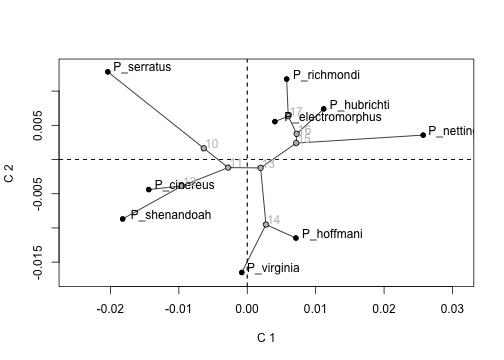
```

![](06-ShapeStatistics1_files/figure-html/unnamed-chunk-39-1.png)
]]

---

### PACA example (alongside PCA example)

+ 9 species of plethodontid salamanders, each with 11 landmarks.

.pull-left[.med[

``` r
summary(PCA)
```
]]

.pull-right[.med[

``` r
summary(PACA)
```
]]

Too much output for one slide but we will see more results in lab.
.med[

**Fraction (of maximum) covariation in each PAC**

```
## Comp1 Comp2 Comp3 Comp4 Comp5 Comp6 Comp7 Comp8 
## 0.099 0.029 0.013 0.007 0.002 0.001 0.000 0.000
```

**Portion variation (.blue[of tips]) in each PAC**

```
## Comp1 Comp2 Comp3 Comp4 Comp5 Comp6 Comp7 Comp8 
## 0.386 0.189 0.190 0.126 0.068 0.026 0.011 0.004
```

**Portion variation (.blue[of tips]) in each PC**

```
## Comp1 Comp2 Comp3 Comp4 Comp5 Comp6 Comp7 Comp8 
## 0.456 0.188 0.182 0.095 0.044 0.021 0.010 0.003
```
]

---

### PACA example (alongside PCA example)

+ 9 species of plethodontid salamanders, each with 11 landmarks.

.pull-left[.med[

``` r
summary(PCA)
```
]]

.pull-right[.med[

``` r
summary(PACA)
```
]]

Too much output for one slide but we will see more results in lab.
.med[

**Fraction (of maximum) covariation in each PAC**

```
## Comp1 Comp2 Comp3 Comp4 Comp5 Comp6 Comp7 Comp8 
## 0.099 0.029 0.013 0.007 0.002 0.001 0.000 0.000
```

**Portion variation (of .red[ancestor values]) in each PAC**

```
## Comp1 Comp2 Comp3 Comp4 Comp5 Comp6 Comp7 Comp8 
## 0.510 0.306 0.101 0.078 0.004 0.000 0.000 0.000
```

**Portion variation (of .red[ancestor values]) in each PC**

```
## Comp1 Comp2 Comp3 Comp4 Comp5 Comp6 Comp7 Comp8 
## 0.385 0.291 0.256 0.040 0.022 0.005 0.001 0.000
```
]

---

### Phylogenetically aligned component analysis (PACA) summary

PACA looks a lot like PCA but with these distinctions:

+ PCA finds maximum variation in first component; PACA finds maximum covariation with *phylogenetic signal* in first few components (more on phylogenetic signal in the **Phylogenetic comparative methods** lecture)
+ PACA will tend to have greater dispersion of *estimated ancestral states* along first PAC than PCA
+ The strength of PACs can be evaluated with partial `$RV$` scores.  (Partial `$RV$` scores in PCA are the portions of variance explained by axes.)

Why use PACA?

+ There are cases where one might wish to visualize evolutionary patterns without obfuscation from other signals (like ecological variation)

---

.center[
# Part V. The General Linear Model

## Alignment of data to hypothesized explanations of variation

]
---

### The General Linear Model
`$$\huge \mathbf{Z}=\mathbf{X}\boldsymbol{\beta } +\mathbf{E}$$`

| Component | Dimension | Description
|------- | :----------- | :-----------------------------
| `$\mathbf{Z}$` | `$n \times p$` | Transformation of a data matrix `$(\mathbf{Y})$` with `$n$` observations for `$p$` variables.  The transformation ***could be*** matrix centering or standardization, but it is also feasible that `$\mathbf{Z} = \mathbf{Y}$`.  **.red[Procrustes coordinates are inherently transformed.]**
| `$\mathbf{X}$` | `$n \times k$` | Linear model design matrix with `$n$` observations for `$k$` parameters
| `$\boldsymbol{\beta}$` | `$k \times p$` | Matrix of coefficients expressing change in values for the `$k$` model parameters for each of `$p$` variables
| `$\mathbf{E}$` | `$n \times p$` | Matrix of residuals (error) for `$n$` observations for `$p$` variables

Like any area of statistics, the coefficients for a linear model (which has parameters for variable change associated with some hypothetical process) are generally unknown but exist in a population, and are, therefore, estimated from a sample.  We can solve this algebraically as the solution that would be true if there was no error in the model (i.e., `$\mathbf{E}$` = 0).  The goal is to solve for `$\boldsymbol{\beta}$`.
---

### The General Linear Model (Cont.)

**Ordinary least-squares estimation (OLS)**

.pull-left[
`$$\small{\mathbf{Z}=\mathbf{X}\boldsymbol{\beta }}$$`
`$$\small{\mathbf{X}^T\mathbf{Z} = \mathbf{X}^T\mathbf{X}\boldsymbol{\beta }}$$`

`$$\small{\left( \mathbf{X}^T\mathbf{X} \right)^{-1} \mathbf{X}^T\mathbf{Z} = 
\left( \mathbf{X}^T\mathbf{X} \right)^{-1} \mathbf{X}^T\mathbf{X}\boldsymbol{\beta }}$$`
`$$\small{\left( \mathbf{X}^T\mathbf{X} \right)^{-1} \mathbf{X}^T\mathbf{Z} = 
\mathbf{I}\boldsymbol{\beta }}$$`

`$$\small{\hat{\boldsymbol{\beta }}=\left ( \mathbf{X}^{T} \mathbf{X}\right )^{-1}\left ( \mathbf{X}^{T} \mathbf{Z}\right )}$$`
]
.pull-right[
The `$\hat{ }$` reminds us that this is a matrix of estimate values.

**Notice that** this resembles something, i.e., `$\hat{\boldsymbol{\beta }}= \mathbf{A}^{T} \mathbf{Z}$`, if `$\mathbf{A} = \mathbf{X}\left ( \mathbf{X}^{T} \mathbf{X}\right )^{-1}$`.

In other words, linear model coefficients are the result of an alignment of data to parameters of a linear model, `$\mathbf{X}$`, which have been standardized by the cross-products of the parameters, `$\left ( \mathbf{X}^{T} \mathbf{X}\right )^{-1}$`.  The matrix `$\mathbf{A}$` in this case is a matrix of standardized model parameters.
]
---

### The General Linear Model (Cont.)

**Generalized least-squares estimation (GLS)**

.pull-left[
`$$\small{\mathbf{Z}=\mathbf{X}\boldsymbol{\beta }}$$`
`$$\small{\mathbf{X}^T \boldsymbol{\Omega}^{-1} \mathbf{Z} = \mathbf{X}^T\boldsymbol{\Omega}^{-1}\mathbf{X}\boldsymbol{\beta }}$$`

`$$\small{\left( \mathbf{X}^T\boldsymbol{\Omega}^{-1}\mathbf{X} \right)^{-1} \mathbf{X}^T\boldsymbol{\Omega}^{-1}\mathbf{Z} = 
\left( \mathbf{X}^T\boldsymbol{\Omega}^{-1}\mathbf{X} \right)^{-1} \mathbf{X}^T\boldsymbol{\Omega}^{-1}\mathbf{X}\boldsymbol{\beta }}$$`
`$$\small{\left( \mathbf{X}^T\boldsymbol{\Omega}^{-1}\mathbf{X} \right)^{-1} \mathbf{X}^T\boldsymbol{\Omega}^{-1}\mathbf{Z} = 
\mathbf{I}\boldsymbol{\beta }}$$`

`$$\small{\hat{\boldsymbol{\beta }}=\left ( \mathbf{X}^{T}\boldsymbol{\Omega}^{-1} \mathbf{X}\right )^{-1}\left ( \mathbf{X}^{T}\boldsymbol{\Omega}^{-1} \mathbf{Z}\right )}$$`
]
.pull-right[
`$\boldsymbol{\Omega}$` is an `$n \times n$` covariance matrix that explains the non-independence among observations.  If `$\boldsymbol{\Omega} = \mathbf{I}$`, then GLS estimation becomes OLS estimation, meaning **observations are independently sampled**.

This is still true: linear model coefficients are the result of an alignment of data to parameters of a linear model, `$\mathbf{X}$`, which have been standardized by the cross-products of the parameter.  However, the standardization of parameter includes accounting for the non-independence among data observations.
]
---

### General Linear Model (Cont.)

**Synthetic approach**

Let `$\boldsymbol{\Omega}^{1/2}$` be a matrix square-root of `$\boldsymbol{\Omega}$`, found either via SVD or a Cholesky decomposition `$^1$`.

Let `$\tilde{\mathbf{X}} = \boldsymbol{\Omega}^{-1/2}\mathbf{X}$`

Let `$\mathbf{\tilde{Z}} = \boldsymbol{\Omega}^{-1/2}\mathbf{Z}$`. `$^2$`

Then,

`$$\hat{\boldsymbol{\beta }}=\left ( \tilde{\mathbf{X}}^{T} \tilde{\mathbf{X}}\right )^{-1}\left ( \tilde{\mathbf{X}}^{T} \mathbf{\tilde{Z}} \right)$$`

.footnote[
1. Different ways of obtaining a matrix square-root are presented in the Appendix.
2. If `$\boldsymbol{\Omega} = \mathbf{I}$`, then `$\mathbf{\tilde{X}} = \mathbf{X}$` and `$\mathbf{\tilde{Z}} = \mathbf{Z}$`, meaning this approach finds either the GLS or OLS solution to estimation.
]

---

### What does a linear model do?

**Regarding coefficients**

1. The coefficients, `$\hat{\boldsymbol{\beta}}$`, explain the expected change in data, `$\mathbf{Z}$`, associated with the *standardized matrix of parameters*.  (This is different than standardizing each of the parameters, which could also be done.)
2. Note that the linear model design has `$k$` parameters (columns).  `$\tilde{\mathbf{X}}^T\tilde{\mathbf{X}}$` is a `$k \times k$` matrix.  `$\mathbf{A} = \tilde{\mathbf{X}}(\tilde{\mathbf{X}}^T\tilde{\mathbf{X}})^{-1}$` is an `$n \times k$` matrix, just like `$\tilde{\mathbf{X}}$`  Thus,

$$ \mathbf{A}^T\mathbf{Z} = \left ( \tilde{\mathbf{X}}^{T} \tilde{\mathbf{X}}\right )^{-1} \tilde{\mathbf{X}}^{T} \mathbf{\tilde{Z}}  = \hat{\boldsymbol{\beta}}$$

`$\hat{\boldsymbol{\beta}}$` is a `$k \times p$` matrix, expressing the change in each of `$p$` variables in `$\mathbf{Z}$` associated with each of `$k$` parameters in `$\tilde{\mathbf{X}}$`.

**This is beautiful just by itself!**

---

**Regarding fitted values, predicted values, and residuals**
4. **Fitted values** are found as `$\hat{\mathbf{Z}} = \mathbf{X}\hat{\boldsymbol{\beta}}$`.  These are made for the full set of data (*training data*) used to estimate coefficients.  **A predicted value** is found as `$\hat{\mathbf{z}}^T_H = \mathbf{x}^T\hat{\boldsymbol{\beta}}$` for any possible vector of model parameters, `$\mathbf{x}^T$`, which might be different than any row vector found in `$\mathbf{X}$`.  The `$_H$` subscript is used to indicate a *hypothetical* result. 
5. **Residuals** are found as `$\mathbf{E} = \mathbf{Z} - \hat{\mathbf{Z}}$`.  If values in `$\mathbf{E}$` tend to be small in magnitude, `$\hat{\mathbf{Z}}$` is close to perfectly estimating `$\mathbf{Z}$`, meaning the model, `$\mathbf{X}$` is *good*.  If values are large, there is much **error** in the model's ability to estimate the data.

.remark-code[.blue[Note that **transformed fitted values** are found as]] `$\hat{\tilde{\mathbf{Z}}} = \tilde{\mathbf{X}}\hat{\boldsymbol{\beta}}$`.

.remark-code[.blue[Note that **transformed residuals** are found as]] `$\tilde{\mathbf{E}} = \tilde{\mathbf{Z}} - \hat{\tilde{\mathbf{Z}}}$`.

Working with transformed fitted values and residuals is important for hypothesis testing.
---

### Let's pause to think about the alignment of data for linear models

All statistical steps take the form, `$\mathbf{A}^T\mathbf{Z}$`, but what `$\mathbf{A}$` comprises changes based on the purpose of the step.

| Step | `$\mathbf{A}$` | `$\mathbf{A}^T$` | Purpose |
|:--|---|---|-----|
|1.| `$\tilde{\mathbf{X}}(\tilde{\mathbf{X}}^T\tilde{\mathbf{X}})^{-1}$`| `$(\tilde{\mathbf{X}}^T\tilde{\mathbf{X}})^{-1}\tilde{\mathbf{X}}^T$` | Obtain coefficients that estimate expected change in `$\mathbf{Z}$` associated with the parameters of `$\mathbf{X}$`, also accounting for the non-independence of observations.|
|2.| `$\mathbf{H} = \mathbf{\tilde{X}} (\tilde{\mathbf{X}}^T\tilde{\mathbf{X}})^{-1}\mathbf{X}^T$` | `$\mathbf{H} = \mathbf{X} (\tilde{\mathbf{X}}^T\tilde{\mathbf{X}})^{-1}\tilde{\mathbf{X}}^T$`| Obtain fitted values.  We can also obtain **.blue[GLS-centered] residuals** as `$\mathbf{E} = \mathbf{Z} -\mathbf{HZ} = (\mathbf{I} - \mathbf{H})\mathbf{Z}$`.|
|3.| `$\tilde{\mathbf{H}} = \mathbf{\mathbf{\tilde{X}}} (\tilde{\mathbf{X}}^T\tilde{\mathbf{X}})^{-1}\tilde{\mathbf{X}}^T$` | `$\tilde{\mathbf{H}} = \tilde{\mathbf{X}} (\tilde{\mathbf{X}}^T\tilde{\mathbf{X}})^{-1}\tilde{\mathbf{X}}^T$`| Obtain **.blue[GLS-transformed] residuals** as `$\tilde{\mathbf{E}} = \mathbf{\tilde{Z}} -\mathbf{\tilde{H}\tilde{Z}} = (\mathbf{ I} - \mathbf{\tilde{H}})\mathbf{\tilde{Z}}$`. .red[The importance of this step is to simply make sure that residuals are transformed for calculating covariance matrices.  This is a bit esoteric, but it will hopefully make some algebraic sense in a moment.] `$^1$`.

.footnote[1. A more extensive explanation of the calculation of GLS-estimated covariance matrices is provided in the Appendix.]

---

### Residual covariance matrices (model error)

+ Residual covariance matrices are the engines that drive statistical analyses.  
+ Residual covariance matrices (or SSCP matrices) are used to estimate ANOVA and MANOVA statistics.
+ Residual covariance matrices can be decomposed to explore patterns of dispersion in the data space.
+ Residual covariance matrices are

`$$\hat{\boldsymbol{\Sigma}} = df^{-1}\mathbf{S} = df^{-1}\tilde{\mathbf{E}}^T\tilde{\mathbf{E}}$$`
+ In other words, covariance matrices are the cross-products of **gls-transformed** residuals, divided by degrees of freedom (mean estimates).
+ If OLS-estimation is used, `$\tilde{\mathbf{E}}= \mathbf{E}$`, as the observations are assumed to be independent.
Presented this way, the algebra is less encumbered than the alternative way, shown in the Appendix.
+ Degrees of freedom `$(df)$` are typically `$n-k$`, where `$n$` is the number of observations and `$k$` is the number of parameters in the model (columns of `$\mathbf{X}$`).
---

### Finally, a linear model example.

**Data:** The `plethShapeFood` data, as used before

**Null model** estimates a mean

**Alternative model** estimates effect of predicting specimen shape from the log of centroid size.  This is accomplished by adding a variable, `$\log(CS)$` to the vector of 1s used to estimate the mean in the linear model design matrix

**OLS analysis.**  Therefore, `$\mathbf{\tilde{X}} = \mathbf{X}$` and `$\mathbf{\tilde{Z}} = \mathbf{Z}$`.

**Set up the analysis and look at `$\mathbf{X}$` matrices.**
The `procD.lm` function is a function that finds a linear model (`.lm`) using Procrustes coordinates (`proc`).  The `D` part is because fitted values can be transcribed into *distances* among predictions in the shape space.

.med[

``` r
data("plethShapeFood")
GPA <- gpagen(plethShapeFood$land, print.progress = FALSE)
fit.null <- procD.lm(coords ~ 1, data = GPA,
                     print.progress = FALSE,
                     iter = 9999)
fit.alt <- procD.lm(coords ~ log(Csize), data = GPA,
                    print.progress = FALSE, 
                    iter = 9999)
```
]

---
### Finally, a linear model example.

**Set up the analysis and look at `$\mathbf{X}$` matrices.**

.pull-left[.med[

``` r
as.matrix(fit.null$LM$X[1:10,])
```

```
##    [,1]
## 1     1
## 2     1
## 3     1
## 4     1
## 5     1
## 6     1
## 7     1
## 8     1
## 9     1
## 10    1
```
]]

.pull-right[.med[

``` r
fit.alt$LM$X[1:10,]
```

```
##    (Intercept) log(Csize)
## 1            1   1.501023
## 2            1   1.415598
## 3            1   1.709488
## 4            1   1.641995
## 5            1   1.409325
## 6            1   1.631807
## 7            1   1.643086
## 8            1   1.551710
## 9            1   1.635676
## 10           1   1.586874
```
]]

---
### Finally, a linear model example.

**Look at the coefficients**

.pull-left[.med[

``` r
coef(fit.null)
```

```
##                   1.X         1.Y       2.X        2.Y        3.X         3.Y
## (Intercept) 0.2415079 -0.07332146 0.2627464 -0.1478185 0.03473031 -0.09093139
##                    4.X       4.Y        5.X        5.Y         6.X          6.Y
## (Intercept) -0.2806804 -0.210035 -0.2896175 -0.1655067 -0.03925596 -0.008809209
##                   7.X          7.Y       8.X       8.Y       9.X        9.Y
## (Intercept) 0.1964961 -0.005244766 0.2489937 0.1166791 0.4406422 0.04415754
##                   10.X       10.Y     11.X      11.Y        12.X     12.Y
## (Intercept) -0.3173787 0.05311804 -0.27118 0.1681822 -0.06589549 0.198903
##                   13.X      13.Y
## (Intercept) -0.1611084 0.1206271
```
]]

.pull-right[.med[

``` r
coef(fit.alt)
```

```
##                    1.X        1.Y        2.X         2.Y         3.X
## (Intercept) 0.20280224 -0.1113977 0.18840275 -0.26478242  0.07183187
## log(Csize)  0.02625426  0.0258273 0.05042762  0.07933718 -0.02516617
##                     3.Y         4.X         4.Y         5.X         5.Y
## (Intercept) -0.10382422 -0.25283896 -0.09617182 -0.24909544 -0.04620803
## log(Csize)   0.00874527 -0.01888499 -0.07723395 -0.02748634 -0.08092083
##                     6.X         6.Y        7.X         7.Y        8.X
## (Intercept) -0.15189901 -0.12482067 0.17906920 -0.04202222 0.19738280
## log(Csize)   0.07640631  0.07869113 0.01182072  0.02494632 0.03500789
##                     8.Y        9.X         9.Y       10.X        10.Y
## (Intercept)  0.22277002  0.6224375  0.14209923 -0.2785311 -0.01523022
## log(Csize)  -0.07196199 -0.1233126 -0.06643432 -0.0263505  0.04636095
##                    11.X       11.Y        12.X        12.Y        13.X
## (Intercept) -0.23733900 0.12470788 -0.06325867  0.27081297 -0.22896415
## log(Csize)  -0.02295454 0.02948886 -0.00178857 -0.04877688  0.04602688
##                   13.Y
## (Intercept) 0.04406722
## log(Csize)  0.05193096
```
]]

---
### Finally, a linear model example.

**Look at the fitted values**

.pull-left[.med[

``` r
fitted(fit.null)[1:5,]
```

```
##         1.X         1.Y       2.X        2.Y        3.X         3.Y        4.X
## 1 0.2415079 -0.07332146 0.2627464 -0.1478185 0.03473031 -0.09093139 -0.2806804
## 2 0.2415079 -0.07332146 0.2627464 -0.1478185 0.03473031 -0.09093139 -0.2806804
## 3 0.2415079 -0.07332146 0.2627464 -0.1478185 0.03473031 -0.09093139 -0.2806804
## 4 0.2415079 -0.07332146 0.2627464 -0.1478185 0.03473031 -0.09093139 -0.2806804
## 5 0.2415079 -0.07332146 0.2627464 -0.1478185 0.03473031 -0.09093139 -0.2806804
##         4.Y        5.X        5.Y         6.X          6.Y       7.X
## 1 -0.210035 -0.2896175 -0.1655067 -0.03925596 -0.008809209 0.1964961
## 2 -0.210035 -0.2896175 -0.1655067 -0.03925596 -0.008809209 0.1964961
## 3 -0.210035 -0.2896175 -0.1655067 -0.03925596 -0.008809209 0.1964961
## 4 -0.210035 -0.2896175 -0.1655067 -0.03925596 -0.008809209 0.1964961
## 5 -0.210035 -0.2896175 -0.1655067 -0.03925596 -0.008809209 0.1964961
##            7.Y       8.X       8.Y       9.X        9.Y       10.X       10.Y
## 1 -0.005244766 0.2489937 0.1166791 0.4406422 0.04415754 -0.3173787 0.05311804
## 2 -0.005244766 0.2489937 0.1166791 0.4406422 0.04415754 -0.3173787 0.05311804
## 3 -0.005244766 0.2489937 0.1166791 0.4406422 0.04415754 -0.3173787 0.05311804
## 4 -0.005244766 0.2489937 0.1166791 0.4406422 0.04415754 -0.3173787 0.05311804
## 5 -0.005244766 0.2489937 0.1166791 0.4406422 0.04415754 -0.3173787 0.05311804
##       11.X      11.Y        12.X     12.Y       13.X      13.Y
## 1 -0.27118 0.1681822 -0.06589549 0.198903 -0.1611084 0.1206271
## 2 -0.27118 0.1681822 -0.06589549 0.198903 -0.1611084 0.1206271
## 3 -0.27118 0.1681822 -0.06589549 0.198903 -0.1611084 0.1206271
## 4 -0.27118 0.1681822 -0.06589549 0.198903 -0.1611084 0.1206271
## 5 -0.27118 0.1681822 -0.06589549 0.198903 -0.1611084 0.1206271
```
]]

.pull-right[.med[

``` r
fitted(fit.alt)[1:5,]
```

```
##         1.X         1.Y       2.X        2.Y        3.X         3.Y        4.X
## 1 0.2422105 -0.07263033 0.2640958 -0.1456955 0.03405687 -0.09069737 -0.2811858
## 2 0.2399677 -0.07483663 0.2597880 -0.1524729 0.03620669 -0.09144443 -0.2795725
## 3 0.2476836 -0.06724624 0.2746082 -0.1291564 0.02881060 -0.08887428 -0.2851226
## 4 0.2459116 -0.06898941 0.2712046 -0.1345112 0.03050915 -0.08946453 -0.2838480
## 5 0.2398030 -0.07499866 0.2594716 -0.1529706 0.03636457 -0.09149930 -0.2794540
##          4.Y        5.X        5.Y         6.X          6.Y       7.X
## 1 -0.2121018 -0.2903531 -0.1676721 -0.03721136 -0.006703465 0.1968124
## 2 -0.2055041 -0.2880050 -0.1607594 -0.04373838 -0.013425668 0.1958026
## 3 -0.2282024 -0.2960830 -0.1845412 -0.02128331  0.009700891 0.1992766
## 4 -0.2229896 -0.2942279 -0.1790796 -0.02644022  0.004389765 0.1984788
## 5 -0.2050195 -0.2878326 -0.1602517 -0.04421770 -0.013919325 0.1957284
##             7.Y       8.X        8.Y       9.X        9.Y       10.X       10.Y
## 1 -0.0045772126 0.2499305 0.11475340 0.4373424 0.04237979 -0.3180838 0.05435864
## 2 -0.0067082562 0.2469399 0.12090076 0.4478764 0.04805495 -0.3158328 0.05039825
## 3  0.0006232258 0.2572284 0.09975183 0.4116361 0.02853055 -0.3235770 0.06402328
## 4 -0.0010604846 0.2548656 0.10460879 0.4199588 0.03301442 -0.3217985 0.06089423
## 5 -0.0068647535 0.2467203 0.12135221 0.4486500 0.04847171 -0.3156675 0.05010741
##         11.X      11.Y        12.X      12.Y       13.X      13.Y
## 1 -0.2717943 0.1689713 -0.06594335 0.1975977 -0.1598767 0.1220168
## 2 -0.2698334 0.1664523 -0.06579056 0.2017645 -0.1638086 0.1175806
## 3 -0.2765795 0.1751187 -0.06631621 0.1874295 -0.1502817 0.1328426
## 4 -0.2750302 0.1731284 -0.06619549 0.1907216 -0.1533883 0.1293376
## 5 -0.2696894 0.1662673 -0.06577934 0.2020705 -0.1640973 0.1172548
```
]]

---
### Finally, a linear model example.

**Look at covariance matrices**

.pull-left[.small[

``` r
Sigma.null <- crossprod(fit.null$LM$residuals)/ (fit.null$LM$n - 
                                     ncol(fit.null$LM$X))
Sigma.null
```

```
##                1.X           1.Y           2.X           2.Y           3.X
## 1.X   8.223585e-05  2.223927e-05  7.670742e-05  3.007037e-05 -1.554810e-05
## 1.Y   2.223927e-05  1.700044e-04  2.068842e-05  1.208913e-04 -6.023450e-06
## 2.X   7.670742e-05  2.068842e-05  1.687747e-04  4.339797e-05 -3.112168e-05
## 2.Y   3.007037e-05  1.208913e-04  4.339797e-05  2.863006e-04 -7.332909e-06
## 3.X  -1.554810e-05 -6.023450e-06 -3.112168e-05 -7.332909e-06  3.001969e-04
## 3.Y  -1.746620e-05  3.248739e-05 -3.603478e-05 -2.506028e-06 -2.482354e-07
## 4.X   1.698994e-05 -3.735893e-05  4.330047e-06 -6.159104e-05 -4.618293e-05
## 4.Y  -1.190757e-04 -1.124586e-04 -1.124424e-04 -1.709534e-04  2.504914e-05
## 5.X   5.972091e-06 -5.221688e-05 -7.630794e-06 -9.769274e-05 -2.152904e-05
## 5.Y  -1.196487e-04 -1.150125e-04 -1.140209e-04 -1.911226e-04  1.785697e-05
## 6.X  -6.392195e-06 -1.724073e-05  4.621300e-05  1.455311e-04  5.241166e-06
## 6.Y   9.920431e-05  9.361213e-05  9.402675e-05  1.104006e-04 -7.210787e-05
## 7.X   8.009168e-06  5.080052e-05  1.701825e-05  4.063765e-05 -6.677471e-05
## 7.Y   3.568162e-05  2.538188e-05  3.066775e-05  1.286461e-05 -8.508957e-05
## 8.X   3.884220e-05  8.577643e-05  4.043354e-05  6.081848e-05 -9.616355e-05
## 8.Y  -6.517590e-05 -1.342166e-04 -1.164575e-04 -1.829886e-04  2.076939e-05
## 9.X  -2.135230e-04 -1.177719e-04 -3.040718e-04 -1.773440e-04 -2.220576e-06
## 9.Y  -8.751944e-05 -1.424854e-04 -6.400493e-05 -1.637553e-04  5.129838e-05
## 10.X -6.239289e-08 -4.718638e-06 -3.756095e-05 -1.521466e-05 -1.436739e-05
## 10.Y  8.462652e-05  1.522471e-05  9.170744e-05  1.242638e-04  4.236651e-05
## 11.X  4.883514e-07  9.915585e-06 -3.063421e-05 -2.971512e-05 -2.879425e-05
## 11.Y  5.489546e-05  3.132705e-05  5.911112e-05  8.257655e-05  4.024204e-05
## 12.X -1.133587e-05  8.195697e-06  5.298752e-06 -1.207794e-05  4.365935e-05
## 12.Y  4.901286e-06 -3.696174e-05  5.527124e-06 -1.058871e-04  2.458260e-05
## 13.X  1.761653e-05  3.771459e-05  5.224371e-05  8.051282e-05 -2.639524e-05
## 13.Y  7.726715e-05  5.220588e-05  9.783385e-05  7.991562e-05 -5.136300e-05
##                3.Y           4.X           4.Y           5.X           5.Y
## 1.X  -1.746620e-05  1.698994e-05 -1.190757e-04  5.972091e-06 -1.196487e-04
## 1.Y   3.248739e-05 -3.735893e-05 -1.124586e-04 -5.221688e-05 -1.150125e-04
## 2.X  -3.603478e-05  4.330047e-06 -1.124424e-04 -7.630794e-06 -1.140209e-04
## 2.Y  -2.506028e-06 -6.159104e-05 -1.709534e-04 -9.769274e-05 -1.911226e-04
## 3.X  -2.482354e-07 -4.618293e-05  2.504914e-05 -2.152904e-05  1.785697e-05
## 3.Y   1.231989e-04 -5.325871e-05 -3.048792e-05 -3.369779e-05 -3.702572e-05
## 4.X  -5.325871e-05  1.896166e-04  2.741338e-05  1.187356e-04  2.522189e-05
## 4.Y  -3.048792e-05  2.741338e-05  2.736439e-04  5.578056e-05  2.558952e-04
## 5.X  -3.369779e-05  1.187356e-04  5.578056e-05  1.401364e-04  4.773574e-05
## 5.Y  -3.702572e-05  2.522189e-05  2.558952e-04  4.773574e-05  3.036677e-04
## 6.X   2.747946e-05 -1.571346e-04 -6.482584e-05 -1.130451e-04 -7.634561e-05
## 6.Y   9.229328e-05 -6.230589e-05 -2.369125e-04 -7.240558e-05 -2.314793e-04
## 7.X  -1.704228e-05  1.600482e-06 -1.527030e-05 -5.372914e-06 -3.139283e-05
## 7.Y   2.336107e-05 -5.107057e-05 -6.862660e-05 -4.512419e-05 -6.060700e-05
## 8.X   2.043250e-05  4.900004e-05 -9.580190e-05 -3.883477e-06 -1.039219e-04
## 8.Y  -1.012850e-05  3.239288e-05  1.816299e-04  5.684229e-05  1.958555e-04
## 9.X   4.465884e-05 -1.050151e-05  3.504589e-04  2.787403e-05  3.885740e-04
## 9.Y  -3.929321e-05 -2.316074e-05  2.234653e-04  1.415791e-05  2.343657e-04
## 10.X -2.365034e-05  6.912470e-06  1.439177e-05 -1.038345e-05  3.065873e-05
## 10.Y -5.477670e-05  3.478209e-06 -1.442827e-04 -1.315831e-05 -1.552684e-04
## 11.X  2.236347e-05 -2.843509e-05 -4.436231e-06 -2.311626e-05  1.686532e-05
## 11.Y -2.509272e-05  4.193944e-05 -1.024696e-04  1.332492e-05 -1.148977e-04
## 12.X  3.837428e-05 -6.181532e-05  2.022270e-05 -2.471898e-05 -9.944447e-06
## 12.Y -6.880383e-05  1.312526e-04  7.565878e-05  1.189317e-04  6.664462e-05
## 13.X  2.808979e-05 -8.311576e-05 -8.146416e-05 -8.303818e-05 -7.163829e-05
## 13.Y -3.226060e-06  2.704753e-05 -1.441017e-04  7.522353e-06 -1.510155e-04
##                6.X           6.Y           7.X           7.Y           8.X
## 1.X  -6.392195e-06  9.920431e-05  8.009168e-06  3.568162e-05  3.884220e-05
## 1.Y  -1.724073e-05  9.361213e-05  5.080052e-05  2.538188e-05  8.577643e-05
## 2.X   4.621300e-05  9.402675e-05  1.701825e-05  3.066775e-05  4.043354e-05
## 2.Y   1.455311e-04  1.104006e-04  4.063765e-05  1.286461e-05  6.081848e-05
## 3.X   5.241166e-06 -7.210787e-05 -6.677471e-05 -8.508957e-05 -9.616355e-05
## 3.Y   2.747946e-05  9.229328e-05 -1.704228e-05  2.336107e-05  2.043250e-05
## 4.X  -1.571346e-04 -6.230589e-05  1.600482e-06 -5.107057e-05  4.900004e-05
## 4.Y  -6.482584e-05 -2.369125e-04 -1.527030e-05 -6.862660e-05 -9.580190e-05
## 5.X  -1.130451e-04 -7.240558e-05 -5.372914e-06 -4.512419e-05 -3.883477e-06
## 5.Y  -7.634561e-05 -2.314793e-04 -3.139283e-05 -6.060700e-05 -1.039219e-04
## 6.X   4.662751e-04  1.008465e-04 -6.422945e-06  5.514742e-05 -1.001202e-04
## 6.Y   1.008465e-04  3.734526e-04 -2.695463e-05  1.592128e-04  1.153018e-04
## 7.X  -6.422945e-06 -2.695463e-05  2.070165e-04 -1.605506e-05  1.164980e-04
## 7.Y   5.514742e-05  1.592128e-04 -1.605506e-05  1.990307e-04  3.008351e-05
## 8.X  -1.001202e-04  1.153018e-04  1.164980e-04  3.008351e-05  3.085628e-04
## 8.Y  -6.630889e-05 -1.508049e-04 -5.661065e-05 -3.665902e-05 -7.279793e-05
## 9.X  -1.064635e-04 -2.461058e-04 -2.113693e-04 -1.689328e-05 -3.035238e-04
## 9.Y  -4.221016e-05 -2.539558e-04 -2.829334e-05 -1.311387e-04 -1.414454e-04
## 10.X -1.077074e-04 -2.888701e-05  1.154908e-05  2.631737e-06 -1.271536e-06
## 10.Y  7.893737e-05  6.728009e-05 -1.930572e-07 -1.442259e-08 -2.231785e-05
## 11.X -7.568846e-05  4.736828e-06 -3.374253e-05  3.565803e-05 -2.593070e-05
## 11.Y  1.844691e-05  1.938303e-05 -1.642128e-06 -3.670103e-05  2.122924e-06
## 12.X  5.100897e-05 -1.881069e-05 -2.009195e-05 -3.383263e-05 -3.903425e-05
## 12.Y -1.476649e-04 -1.499941e-04  4.604932e-05 -9.814991e-05  7.590249e-06
## 13.X  1.042362e-04  1.134613e-04 -1.791710e-05  5.819522e-05  1.659097e-05
## 13.Y -1.179266e-05  1.075121e-04  5.596677e-05  1.204568e-05  1.141591e-04
##                8.Y           9.X           9.Y          10.X          10.Y
## 1.X  -6.517590e-05 -2.135230e-04 -8.751944e-05 -6.239289e-08  8.462652e-05
## 1.Y  -1.342166e-04 -1.177719e-04 -1.424854e-04 -4.718638e-06  1.522471e-05
## 2.X  -1.164575e-04 -3.040718e-04 -6.400493e-05 -3.756095e-05  9.170744e-05
## 2.Y  -1.829886e-04 -1.773440e-04 -1.637553e-04 -1.521466e-05  1.242638e-04
## 3.X   2.076939e-05 -2.220576e-06  5.129838e-05 -1.436739e-05  4.236651e-05
## 3.Y  -1.012850e-05  4.465884e-05 -3.929321e-05 -2.365034e-05 -5.477670e-05
## 4.X   3.239288e-05 -1.050151e-05 -2.316074e-05  6.912470e-06  3.478209e-06
## 4.Y   1.816299e-04  3.504589e-04  2.234653e-04  1.439177e-05 -1.442827e-04
## 5.X   5.684229e-05  2.787403e-05  1.415791e-05 -1.038345e-05 -1.315831e-05
## 5.Y   1.958555e-04  3.885740e-04  2.343657e-04  3.065873e-05 -1.552684e-04
## 6.X  -6.630889e-05 -1.064635e-04 -4.221016e-05 -1.077074e-04  7.893737e-05
## 6.Y  -1.508049e-04 -2.461058e-04 -2.539558e-04 -2.888701e-05  6.728009e-05
## 7.X  -5.661065e-05 -2.113693e-04 -2.829334e-05  1.154908e-05 -1.930572e-07
## 7.Y  -3.665902e-05 -1.689328e-05 -1.311387e-04  2.631737e-06 -1.442259e-08
## 8.X  -7.279793e-05 -3.035238e-04 -1.414454e-04 -1.271536e-06 -2.231785e-05
## 8.Y   2.787883e-04  2.669630e-04  1.261995e-04  1.756680e-05 -1.149388e-04
## 9.X   2.669630e-04  1.030986e-03  2.650311e-04  1.044193e-04 -2.227181e-04
## 9.Y   1.261995e-04  2.650311e-04  3.604643e-04  2.147813e-05 -6.267501e-05
## 10.X  1.756680e-05  1.044193e-04  2.147813e-05  1.376990e-04 -1.718805e-05
## 10.Y -1.149388e-04 -2.227181e-04 -6.267501e-05 -1.718805e-05  2.339593e-04
## 11.X  1.508028e-05  1.393613e-04  2.410029e-05  5.026614e-05 -1.906190e-05
## 11.Y -8.016111e-05 -1.848726e-04 -6.873774e-05 -1.111171e-05  8.693827e-05
## 12.X  2.519972e-05 -6.310494e-05  6.706324e-05 -8.706290e-05 -2.350484e-05
## 12.Y  4.757829e-05 -6.287741e-05  4.530247e-05  1.883077e-05 -4.766539e-05
## 13.X -5.746349e-05 -8.786193e-05 -5.649496e-05 -5.243000e-05  1.702604e-05
## 13.Y -1.201541e-04 -2.871027e-04 -1.277563e-04 -4.787519e-06  5.195532e-05
##               11.X          11.Y          12.X          12.Y          13.X
## 1.X   4.883514e-07  5.489546e-05 -1.133587e-05  4.901286e-06  1.761653e-05
## 1.Y   9.915585e-06  3.132705e-05  8.195697e-06 -3.696174e-05  3.771459e-05
## 2.X  -3.063421e-05  5.911112e-05  5.298752e-06  5.527124e-06  5.224371e-05
## 2.Y  -2.971512e-05  8.257655e-05 -1.207794e-05 -1.058871e-04  8.051282e-05
## 3.X  -2.879425e-05  4.024204e-05  4.365935e-05  2.458260e-05 -2.639524e-05
## 3.Y   2.236347e-05 -2.509272e-05  3.837428e-05 -6.880383e-05  2.808979e-05
## 4.X  -2.843509e-05  4.193944e-05 -6.181532e-05  1.312526e-04 -8.311576e-05
## 4.Y  -4.436231e-06 -1.024696e-04  2.022270e-05  7.565878e-05 -8.146416e-05
## 5.X  -2.311626e-05  1.332492e-05 -2.471898e-05  1.189317e-04 -8.303818e-05
## 5.Y   1.686532e-05 -1.148977e-04 -9.944447e-06  6.664462e-05 -7.163829e-05
## 6.X  -7.568846e-05  1.844691e-05  5.100897e-05 -1.476649e-04  1.042362e-04
## 6.Y   4.736828e-06  1.938303e-05 -1.881069e-05 -1.499941e-04  1.134613e-04
## 7.X  -3.374253e-05 -1.642128e-06 -2.009195e-05  4.604932e-05 -1.791710e-05
## 7.Y   3.565803e-05 -3.670103e-05 -3.383263e-05 -9.814991e-05  5.819522e-05
## 8.X  -2.593070e-05  2.122924e-06 -3.903425e-05  7.590249e-06  1.659097e-05
## 8.Y   1.508028e-05 -8.016111e-05  2.519972e-05  4.757829e-05 -5.746349e-05
## 9.X   1.393613e-04 -1.848726e-04 -6.310494e-05 -6.287741e-05 -8.786193e-05
## 9.Y   2.410029e-05 -6.873774e-05  6.706324e-05  4.530247e-05 -5.649496e-05
## 10.X  5.026614e-05 -1.111171e-05 -8.706290e-05  1.883077e-05 -5.243000e-05
## 10.Y -1.906190e-05  8.693827e-05 -2.350484e-05 -4.766539e-05  1.702604e-05
## 11.X  1.231055e-04 -3.414632e-05 -6.370426e-05 -3.874634e-05 -3.175538e-06
## 11.Y -3.414632e-05  1.340429e-04  7.947113e-06  2.735202e-05 -6.257145e-06
## 12.X -6.370426e-05  7.947113e-06  2.603858e-04 -4.878231e-06  1.051563e-05
## 12.Y -3.874634e-05  2.735202e-05 -4.878231e-06  2.368705e-04 -1.034987e-04
## 13.X -3.175538e-06 -6.257145e-06  1.051563e-05 -1.034987e-04  1.527307e-04
## 13.Y -2.613899e-06  4.644012e-05 -6.395397e-05  8.055436e-06  4.181705e-05
##               13.Y
## 1.X   7.726715e-05
## 1.Y   5.220588e-05
## 2.X   9.783385e-05
## 2.Y   7.991562e-05
## 3.X  -5.136300e-05
## 3.Y  -3.226060e-06
## 4.X   2.704753e-05
## 4.Y  -1.441017e-04
## 5.X   7.522353e-06
## 5.Y  -1.510155e-04
## 6.X  -1.179266e-05
## 6.Y   1.075121e-04
## 7.X   5.596677e-05
## 7.Y   1.204568e-05
## 8.X   1.141591e-04
## 8.Y  -1.201541e-04
## 9.X  -2.871027e-04
## 9.Y  -1.277563e-04
## 10.X -4.787519e-06
## 10.Y  5.195532e-05
## 11.X -2.613899e-06
## 11.Y  4.644012e-05
## 12.X -6.395397e-05
## 12.Y  8.055436e-06
## 13.X  4.181705e-05
## 13.Y  1.881235e-04
```
]]

.pull-right[.small[

``` r
Sigma.alt <- crossprod(fit.alt$LM$residuals)/ (fit.alt$LM$n - 
                                     ncol(fit.alt$LM$X))
Sigma.alt
```

```
##                1.X           1.Y           2.X           2.Y           3.X
## 1.X   6.866299e-05  8.011630e-06  4.942485e-05 -1.420540e-05 -1.593285e-06
## 1.Y   8.011630e-06  1.582190e-04 -6.967949e-06  7.869843e-05  7.842806e-06
## 2.X   4.942485e-05 -6.967949e-06  1.166920e-04 -4.185861e-05 -4.336882e-06
## 2.Y  -1.420540e-05  7.869843e-05 -4.185861e-05  1.554214e-04  3.542865e-05
## 3.X  -1.593285e-06  7.842806e-06 -4.336882e-06  3.542865e-05  2.910786e-04
## 3.Y  -2.265684e-05  2.812250e-05 -4.604178e-05 -1.744115e-05  4.473694e-06
## 4.X   2.788952e-05 -2.744366e-05  2.484287e-05 -3.033940e-05 -5.707701e-05
## 4.Y  -7.731403e-05 -7.130625e-05 -3.049361e-05 -4.193553e-05 -1.631149e-05
## 5.X   2.155604e-05 -3.775341e-05  2.201683e-05 -5.232739e-05 -3.670301e-05
## 5.Y  -7.581719e-05 -7.185359e-05 -2.810364e-05 -5.612516e-05 -2.560325e-05
## 6.X  -4.955997e-05 -5.986996e-05 -3.582810e-05  1.754376e-05  4.660666e-05
## 6.Y   5.632458e-05  5.137035e-05  1.022534e-05 -2.200330e-05 -3.066221e-05
## 7.X   1.465040e-06  4.500344e-05  4.473079e-06  2.110739e-05 -6.138385e-05
## 7.Y   2.215124e-05  1.192648e-05  4.114223e-06 -2.943988e-05 -7.287945e-05
## 8.X   1.968701e-05  6.764269e-05  3.131358e-06  2.089674e-06 -7.868180e-05
## 8.Y  -2.558169e-05 -9.631254e-05 -4.027699e-05 -6.313131e-05 -1.780633e-05
## 9.X  -1.471952e-04 -5.114543e-05 -1.750904e-04  3.007416e-05 -6.888747e-05
## 9.Y  -5.137482e-05 -1.077702e-04  6.973188e-06 -5.302741e-05  1.616527e-05
## 10.X  1.479119e-05  9.823872e-06 -9.589905e-06  2.944677e-05 -2.882071e-05
## 10.Y  5.975464e-05 -1.025800e-05  4.287773e-05  4.714178e-05  6.805066e-05
## 11.X  1.343576e-05  2.279325e-05 -6.236834e-06  8.944831e-06 -4.162784e-05
## 11.Y  3.909110e-05  1.544127e-05  2.806357e-05  3.357425e-05  5.677740e-05
## 12.X -1.049680e-05  9.309891e-06  7.314457e-06 -9.211351e-06  4.334450e-05
## 12.Y  3.247133e-05 -1.046369e-05  5.842401e-05 -2.437529e-05 -1.407794e-06
## 13.X -8.067174e-06  1.275282e-05  3.186710e-06  3.306924e-06 -1.917900e-06
## 13.Y  4.914546e-05  2.418623e-05  4.306452e-05 -7.356890e-06 -2.406796e-05
##                3.Y           4.X           4.Y           5.X           5.Y
## 1.X  -2.265684e-05  2.788952e-05 -7.731403e-05  2.155604e-05 -7.581719e-05
## 1.Y   2.812250e-05 -2.744366e-05 -7.130625e-05 -3.775341e-05 -7.185359e-05
## 2.X  -4.604178e-05  2.484287e-05 -3.049361e-05  2.201683e-05 -2.810364e-05
## 2.Y  -1.744115e-05 -3.033940e-05 -4.193553e-05 -5.232739e-05 -5.612516e-05
## 3.X   4.473694e-06 -5.707701e-05 -1.631149e-05 -3.670301e-05 -2.560325e-05
## 3.Y   1.233956e-04 -5.050745e-05 -1.644018e-05 -2.903943e-05 -2.238325e-05
## 4.X  -5.050745e-05  1.847889e-04 -3.495531e-06  1.093622e-04 -7.214739e-06
## 4.Y  -1.644018e-05 -3.495531e-06  1.496467e-04  1.103095e-05  1.255189e-04
## 5.X  -2.903943e-05  1.093622e-04  1.103095e-05  1.260060e-04  6.901293e-07
## 5.Y  -2.238325e-05 -7.214739e-06  1.255189e-04  6.901293e-07  1.675984e-04
## 6.X   1.354224e-05 -1.284975e-04  6.091556e-05 -6.963861e-05  5.527248e-05
## 6.Y   7.889439e-05 -3.132689e-05 -1.099505e-04 -2.704410e-05 -9.820676e-05
## 7.X  -1.951630e-05  6.417624e-06  4.104755e-06  1.523278e-06 -1.132263e-05
## 7.Y   1.902539e-05 -4.171718e-05 -2.828097e-05 -3.107479e-05 -1.816682e-05
## 8.X   1.416378e-05  6.392695e-05 -3.917620e-05  1.671962e-05 -4.464599e-05
## 8.Y   3.233150e-06  3.696048e-06  6.500211e-05  1.521994e-05  7.374324e-05
## 9.X   6.848069e-05 -6.066101e-05  1.511934e-04 -4.448691e-05  1.801154e-04
## 9.Y  -2.740483e-05 -5.044528e-05  1.166288e-04 -2.483917e-05  1.224327e-04
## 10.X -1.905531e-05 -3.669380e-06 -2.909195e-05 -2.609004e-05 -1.466822e-05
## 10.Y -6.429980e-05  2.232931e-05 -6.955320e-05  1.400674e-05 -7.703274e-05
## 11.X  2.700760e-05 -3.816747e-05 -4.256926e-05 -3.700865e-05 -2.276695e-05
## 11.Y -3.100457e-05  5.452302e-05 -5.509597e-05  3.092762e-05 -6.537510e-05
## 12.X  3.928288e-05 -6.346320e-05  1.755845e-05 -2.614351e-05 -1.320055e-05
## 12.Y -6.067156e-05  1.134327e-04 -4.101467e-06  9.191952e-05 -1.711154e-05
## 13.X  1.986624e-05 -6.569257e-05 -6.351048e-06 -5.711328e-05  7.265144e-06
## 13.Y -1.302566e-05  4.850902e-05 -6.013243e-05  3.828339e-05 -6.303831e-05
##                6.X           6.Y           7.X           7.Y           8.X
## 1.X  -4.955997e-05  5.632458e-05  1.465040e-06  2.215124e-05  1.968701e-05
## 1.Y  -5.986996e-05  5.137035e-05  4.500344e-05  1.192648e-05  6.764269e-05
## 2.X  -3.582810e-05  1.022534e-05  4.473079e-06  4.114223e-06  3.131358e-06
## 2.Y   1.754376e-05 -2.200330e-05  2.110739e-05 -2.943988e-05  2.089674e-06
## 3.X   4.660666e-05 -3.066221e-05 -6.138385e-05 -7.287945e-05 -7.868180e-05
## 3.Y   1.354224e-05  7.889439e-05 -1.951630e-05  1.902539e-05  1.416378e-05
## 4.X  -1.284975e-04 -3.132689e-05  6.417624e-06 -4.171718e-05  6.392695e-05
## 4.Y   6.091556e-05 -1.099505e-04  4.104755e-06 -2.828097e-05 -3.917620e-05
## 5.X  -6.963861e-05 -2.704410e-05  1.523278e-06 -3.107479e-05  1.671962e-05
## 5.Y   5.527248e-05 -9.820676e-05 -1.132263e-05 -1.816682e-05 -4.464599e-05
## 6.X   3.478833e-04 -2.674789e-05 -2.591171e-05  1.504392e-05 -1.590480e-04
## 6.Y  -2.674789e-05  2.460664e-04 -4.732976e-05  1.194386e-04  5.787180e-05
## 7.X  -2.591171e-05 -4.732976e-05  2.071061e-04 -2.262638e-05  1.093513e-04
## 7.Y   1.504392e-05  1.194386e-04 -2.262638e-05  1.886389e-04  1.178076e-05
## 8.X  -1.590480e-04  5.787180e-05  1.093513e-04  1.178076e-05  2.868533e-04
## 8.Y   5.076127e-05 -3.146543e-05 -3.919071e-05  1.339846e-06 -1.979174e-05
## 9.X   9.425233e-05 -4.142450e-05 -1.832258e-04  4.890623e-05 -2.153618e-04
## 9.Y   6.615104e-05 -1.454957e-04 -1.185374e-05 -9.751084e-05 -9.361890e-05
## 10.X -6.608473e-05  1.520483e-05  1.840955e-05  1.678550e-05  1.851675e-05
## 10.Y  4.056403e-06 -1.004930e-05 -1.196294e-05 -2.484761e-05 -5.749977e-05
## 11.X -3.915924e-05  4.359256e-05 -2.841999e-05  4.848570e-05 -9.063147e-06
## 11.Y -2.965678e-05 -3.015339e-05 -9.151289e-06 -5.304434e-05 -2.001171e-05
## 12.X  5.470460e-05 -1.606940e-05 -1.993787e-05 -3.337955e-05 -3.827241e-05
## 12.Y -6.984619e-05 -6.981722e-05  5.911682e-05 -7.348778e-05  4.436837e-05
## 13.X  3.028095e-05  3.738564e-05 -2.986674e-05  3.440979e-05 -1.775909e-05
## 13.Y -9.716587e-05  2.137185e-05  4.362135e-05 -1.559104e-05  7.682725e-05
##                8.Y           9.X           9.Y          10.X          10.Y
## 1.X  -2.558169e-05 -1.471952e-04 -5.137482e-05  1.479119e-05  5.975464e-05
## 1.Y  -9.631254e-05 -5.114543e-05 -1.077702e-04  9.823872e-06 -1.025800e-05
## 2.X  -4.027699e-05 -1.750904e-04  6.973188e-06 -9.589905e-06  4.287773e-05
## 2.Y  -6.313131e-05  3.007416e-05 -5.302741e-05  2.944677e-05  4.714178e-05
## 3.X  -1.780633e-05 -6.888747e-05  1.616527e-05 -2.882071e-05  6.805066e-05
## 3.Y   3.233150e-06  6.848069e-05 -2.740483e-05 -1.905531e-05 -6.429980e-05
## 4.X   3.696048e-06 -6.066101e-05 -5.044528e-05 -3.669380e-06  2.232931e-05
## 4.Y   6.500211e-05  1.511934e-04  1.166288e-04 -2.909195e-05 -6.955320e-05
## 5.X   1.521994e-05 -4.448691e-05 -2.483917e-05 -2.609004e-05  1.400674e-05
## 5.Y   7.374324e-05  1.801154e-04  1.224327e-04 -1.466822e-05 -7.703274e-05
## 6.X   5.076127e-05  9.425233e-05  6.615104e-05 -6.608473e-05  4.056403e-06
## 6.Y  -3.146543e-05 -4.142450e-05 -1.454957e-04  1.520483e-05 -1.004930e-05
## 7.X  -3.919071e-05 -1.832258e-04 -1.185374e-05  1.840955e-05 -1.196294e-05
## 7.Y   1.339846e-06  4.890623e-05 -9.751084e-05  1.678550e-05 -2.484761e-05
## 8.X  -1.979174e-05 -2.153618e-04 -9.361890e-05  1.851675e-05 -5.749977e-05
## 8.Y   1.717567e-04  8.041007e-05  2.543159e-05 -2.288669e-05 -4.501932e-05
## 9.X   8.041007e-05  7.198727e-04  9.308524e-05  3.620825e-05 -1.032900e-04
## 9.Y   2.543159e-05  9.308524e-05  2.710779e-04 -1.578946e-05  2.521987e-06
## 10.X -2.288669e-05  3.620825e-05 -1.578946e-05  1.248453e-04  8.786171e-06
## 10.Y -4.501932e-05 -1.032900e-04  2.521987e-06  8.786171e-06  1.913010e-04
## 11.X -2.016303e-05  8.066345e-05 -8.283938e-06  3.802884e-05  3.503832e-06
## 11.Y -3.579259e-05 -1.095528e-04 -2.769874e-05  5.407074e-06  5.888099e-05
## 12.X  2.281221e-05 -6.878250e-05  6.551285e-05 -8.937430e-05 -2.207522e-05
## 12.Y -2.707959e-05 -1.929649e-04 -2.360007e-05 -8.485860e-06  1.784357e-07
## 13.X  1.279765e-05  3.269440e-05  8.317724e-06 -2.717080e-05 -2.853757e-05
## 13.Y -4.170586e-05 -1.538876e-04 -5.558524e-05  2.452326e-05  1.035789e-06
##               11.X          11.Y          12.X          12.Y          13.X
## 1.X   1.343576e-05  3.909110e-05 -1.049680e-05  3.247133e-05 -8.067174e-06
## 1.Y   2.279325e-05  1.544127e-05  9.309891e-06 -1.046369e-05  1.275282e-05
## 2.X  -6.236834e-06  2.806357e-05  7.314457e-06  5.842401e-05  3.186710e-06
## 2.Y   8.944831e-06  3.357425e-05 -9.211351e-06 -2.437529e-05  3.306924e-06
## 3.X  -4.162784e-05  5.677740e-05  4.334450e-05 -1.407794e-06 -1.917900e-06
## 3.Y   2.700760e-05 -3.100457e-05  3.928288e-05 -6.067156e-05  1.986624e-05
## 4.X  -3.816747e-05  5.452302e-05 -6.346320e-05  1.134327e-04 -6.569257e-05
## 4.Y  -4.256926e-05 -5.509597e-05  1.755845e-05 -4.101467e-06 -6.351048e-06
## 5.X  -3.700865e-05  3.092762e-05 -2.614351e-05  9.191952e-05 -5.711328e-05
## 5.Y  -2.276695e-05 -6.537510e-05 -1.320055e-05 -1.711154e-05  7.265144e-06
## 6.X  -3.915924e-05 -2.965678e-05  5.470460e-05 -6.984619e-05  3.028095e-05
## 6.Y   4.359256e-05 -3.015339e-05 -1.606940e-05 -6.981722e-05  3.738564e-05
## 7.X  -2.841999e-05 -9.151289e-06 -1.993787e-05  5.911682e-05 -2.986674e-05
## 7.Y   4.848570e-05 -5.304434e-05 -3.337955e-05 -7.348778e-05  3.440979e-05
## 8.X  -9.063147e-06 -2.001171e-05 -3.827241e-05  4.436837e-05 -1.775909e-05
## 8.Y  -2.016303e-05 -3.579259e-05  2.281221e-05 -2.707959e-05  1.279765e-05
## 9.X   8.066345e-05 -1.095528e-04 -6.878250e-05 -1.929649e-04  3.269440e-05
## 9.Y  -8.283938e-06 -2.769874e-05  6.551285e-05 -2.360007e-05  8.317724e-06
## 10.X  3.802884e-05  5.407074e-06 -8.937430e-05 -8.485860e-06 -2.717080e-05
## 10.Y  3.503832e-06  5.888099e-05 -2.207522e-05  1.784357e-07 -2.853757e-05
## 11.X  1.136291e-04 -2.012159e-05 -6.553661e-05 -6.336564e-05  1.946264e-05
## 11.Y -2.012159e-05  1.173718e-04  9.198215e-06  5.864485e-05 -3.549387e-05
## 12.X -6.553661e-05  9.198215e-06  2.642034e-04 -6.824265e-06  1.244019e-05
## 12.Y -6.336564e-05  5.864485e-05 -6.824265e-06  1.893204e-04 -5.683814e-05
## 13.X  1.946264e-05 -3.549387e-05  1.244019e-05 -5.683814e-05  1.095227e-04
## 13.Y  2.294265e-05  1.425157e-05 -6.291415e-05  6.256455e-05 -8.881288e-06
##               13.Y
## 1.X   4.914546e-05
## 1.Y   2.418623e-05
## 2.X   4.306452e-05
## 2.Y  -7.356890e-06
## 3.X  -2.406796e-05
## 3.Y  -1.302566e-05
## 4.X   4.850902e-05
## 4.Y  -6.013243e-05
## 5.X   3.828339e-05
## 5.Y  -6.303831e-05
## 6.X  -9.716587e-05
## 6.Y   2.137185e-05
## 7.X   4.362135e-05
## 7.Y  -1.559104e-05
## 8.X   7.682725e-05
## 8.Y  -4.170586e-05
## 9.X  -1.538876e-04
## 9.Y  -5.558524e-05
## 10.X  2.452326e-05
## 10.Y  1.035789e-06
## 11.X  2.294265e-05
## 11.Y  1.425157e-05
## 12.X -6.291415e-05
## 12.Y  6.256455e-05
## 13.X -8.881288e-06
## 13.Y  1.330255e-04
```
]]

---
### Finally, a linear model example.

**Look at covariance matrices**

Obviously in the previous illustration, we cannot easily make sense of the difference between covariance matrices, but we can see that the diagonal of the second matrix had decreased values, meaning the residual variances (of each of the variables) is decreasing by adding `$\log(CS)$` to the linear model.  **We are explaining more variation in the data with an additional parameter.**

We can summarize the combined changes between the two matrices with, 
`$trace(\hat{\boldsymbol{\Sigma}}_{effect})$`, which is found one of two ways:

.pull-left[.small[.pre[
*Constructing the covariance matrix for the effect from the residual covariance matrices*

``` r
sum(diag(Sigma.null * (fit.null$LM$n -ncol(fit.null$LM$X)) - 
           Sigma.alt * (fit.alt$LM$n -ncol(fit.alt$LM$X)))) / 
  (ncol(fit.alt$LM$X) - ncol(fit.null$LM$X))
```

```
## [1] 0.1075834
```
]]]

.pull-right[.small[.pre[
*Constructing the covariance matrix for the effect from the fitted values*

``` r
Sigma.effect <- (crossprod(fitted(fit.alt) - fitted(fit.null))) /
  (ncol(fit.alt$LM$X) - ncol(fit.null$LM$X))
sum(diag(Sigma.effect))
```

```
## [1] 0.1075834
```
]]]

.red[Yes, the code is ugly, but shows we get the same value whether we compare the residual covariance matrices or the cross-products of fitted values.]
---
### Finally, a linear model example.

**Notice something familiar?**
.pull-left[.small[.pre[

``` r
anova(fit.alt)
```

```
## 
## Analysis of Variance, using Residual Randomization
## Permutation procedure: Randomization of null model residuals 
## Number of permutations: 10000 
## Estimation method: Ordinary Least Squares 
## Sums of Squares and Cross-products: Type I 
## Effect sizes (Z) based on F distributions
## 
##            Df      SS       MS     Rsq      F      Z Pr(>F)    
## log(Csize)  1 0.10758 0.107583 0.23511 20.594 5.3289  1e-04 ***
## Residuals  67 0.35001 0.005224 0.76489                         
## Total      68 0.45759                                          
## ---
## Signif. codes:  0 '***' 0.001 '**' 0.01 '*' 0.05 '.' 0.1 ' ' 1
## 
## Call: procD.lm(f1 = coords ~ log(Csize), iter = 9999, data = GPA, print.progress = FALSE)
```
]]]

.pull-left[.med[.pre[

``` r
summary(PLSallometry)
```

---
### General linear model summary

+ If we follow the paradigm that `$\mathbf{A}^T\mathbf{Z}$` is the general method of alignment of data for a specific statistical purpose,
  + If `$\mathbf{A}$` is a matrix of standardized model parameters, linear model coefficients are produced.
  + If `$\mathbf{A}$` is a hat matrix `$(\mathbf{H})$`, fitted values are produced.
  + If `$\mathbf{A}$` is a transformed hat matrix `$(\mathbf{\tilde{H}})$`, transformed fitted values are produced and can be used to estimate covariance matrices.
  + Covariance matrices allow models to be compared, which means statistical evaluation is needed (e.g., with RRPP).
  
### We did not get into statistical evaluation with linear models.

+ This will be done in the **Shape Statistics II** lecture.
+ Here's a hint: RRPP means we can estimate many (thousands) of random covariance matrices and derive from them sampling distributions of statistics.  We saw one example: `$MS = trace(\hat{\boldsymbol{\Sigma}})$`.
---

### A more general summary, for what `$\mathbf{A}^T\mathbf{Z}$` means

`$\mathbf{A}^T\mathbf{Z}$` describes the alignment of data `$(\mathbf{Z})$` to something `$(\mathbf{A})$`.  The product above can be either (1) decomposed or (2) compared to alternative alignments.  The table below summarizes the analyses we have covered, whether decomposition or comparison is prominent, and their purpose.

|Analysis| `$(\mathbf{A})$` |Treatment|Purpose|
|---|---|---|---|
|PCA| `$\mathbf{I}$` |Decompose|Find the principal vectors of variation in a multivariate data space, to best envision patterns of dispersion|
|PLS| `$\mathbf{Z}_{other}$` |Decompose| Find the principal vectors of covariation between two data sets.  Statistical analysis is also possible by creating random distributions of correlation coefficients between principal scores.|
|PACA| `$\boldsymbol{\Omega}$` |Decompose|Find the principal vectors of variation in a multivariate data space, constrained to be aligned with phylogenetic signal.  PACs might be similar to PCs if phylogenetic signal pervades shape differences.  PACs could be different if other sources of variation exist.|
|GLM| `$\mathbf{H}$` |Compare|Find the coefficients and fitted values of null and alternative models, and compare the alternative to the null to ascertain whether parameters are meaningful.|

All of these purposes are helpful for inferential statistics, the more prominent theme in **Shape Statistics II**.

---

### Revisiting Linear Algebra Goals
.pull-left[.med[

`$$\small\mathbf{Z}=[trace[\mathbf{(Y-\overline{Y})(Y-\overline{Y})^T}]]^{-1/2}\mathbf{(Y-\overline{Y})H}$$`

**Should be more obvious now, although it probably looks more obvious as `$\small\mathbf{Z}=CS^{-1}\mathbf{(Y-\overline{Y})H}$`**.

Procrustes coordinates: linear transformation of coordinate data.

----

`$$\hat{\boldsymbol{\beta}}=\left ( \mathbf{\tilde{X}}^{T} \mathbf{\tilde{X}}\right )^{-1}\left ( \mathbf{\tilde{X}}^{T} \mathbf{\tilde{Z}}\right )$$`

**Estimation of linear model coefficients for transformed data, `$\mathbf{Z}$`, which Procrustes coordinates are.**

Coefficients:  transformation of the data, based on model parameters.

----
]]

.pull-right[.med[

`$$\mathbf{A}^T\mathbf{Z} =\mathbf{UDV}^T$$`

The decomposition of some form of data alignment: hopefully this makes sense now!

]]